

Hypothesis Testing#
Michael J. Pyrcz, Professor, The University of Texas at Austin
Twitter | GitHub | Website | GoogleScholar | Geostatistics Book | YouTube | Applied Geostats in Python e-book | Applied Machine Learning in Python e-book | LinkedIn
Chapter of e-book “Applied Geostatistics in Python: a Hands-on Guide with GeostatsPy”.
Cite this e-Book as:
Pyrcz, M.J., 2024, Applied Geostatistics in Python: a Hands-on Guide with GeostatsPy [e-book]. Zenodo. doi:10.5281/zenodo.15169133 ![]()
The workflows in this book and more are available here:
Cite the GeostatsPyDemos GitHub Repository as:
Pyrcz, M.J., 2024, GeostatsPyDemos: GeostatsPy Python Package for Spatial Data Analytics and Geostatistics Demonstration Workflows Repository (0.0.1) [Software]. Zenodo. doi:10.5281/zenodo.12667036. GitHub Repository: GeostatsGuy/GeostatsPyDemos ![]()
By Michael J. Pyrcz
© Copyright 2024.
This chapter is a tutorial for / demonstration of Hypothesis Testing.
YouTube Lecture: check out my lectures on:
Motivation for Hypothesis Testing#
We need to report uncertainty and significance of our results! Otherwise, we do not know if any of our results are meaningful. For example, if we collected 2 sample sets, one from well 1 and the other from well 2, we will want to know if the difference in the means are,
statistically significant - suggesting that we may sampled 2 distinct populations
statistically insignificant - suggesting that we may be sampling the same population (with respect to the mean)
We will take all the related information, for example, sample means, sample standard deviations, and number of samples and calculate the expected distribution of difference assuming the same population and then calculate the critical values that if exceeded indicate a significant difference.
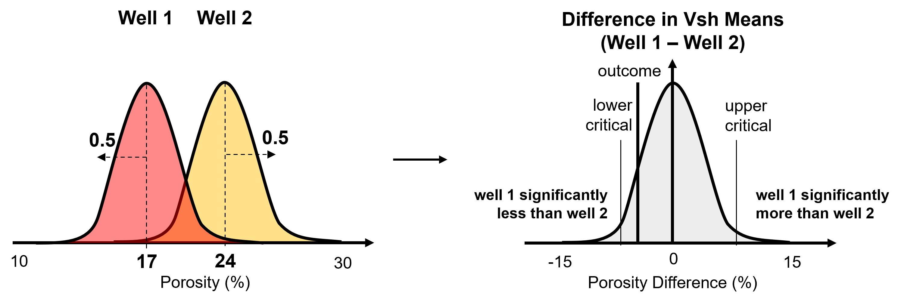
this is an illustration of the hypothesis testing approach that is not completely accurate (i.e., our sampling distribution is in standardized difference and not in difference), but communicates the concepts.
Hypothesis Testing Concepts#
To understand hypothesis testing, we must understand the following concepts. Let’s start with the hypothesis,
Hypothesis- a statement about a population parameter, for example, \(\mu_1 = \mu_2\). Note, we never use sample statistics, for example, \(\overline{X_1} = \overline{X_2}\), because we know the sample statistics and there is no need to make any inference concerning them.
We start by accepting the null hypothesis, \(H_0\), and then test it.
Null Hypothesis (\(H0\)) and Alternative Hypothesis (\(H1\)) - two complementary hypotheses in a hypothesis testing problem
\(H_0\) – no effect, e.g. means are the same, one is not larger, difference due to limited samples and random effect
\(H_1\) – a significant difference, the effect we are checking for
To test the null hypothesis we calculate the,
Sampling Distribution - the theoretical distributions given the null hypothesis is true, for example,
Student’s t - for Student’s t‐test for comparing the means of two sample sets
F‐distribution - for the F-test for Comparing the variances of two sample sets
Chi‐Square distribution - for CHi-square test for comparing entire histograms of two sample sets
statistic - a measure of difference in units of standard deviations from the 0 difference, generally calculated as the measure divided by standard error. The measure is the difference, for example, the difference in the means. Standard error integrates information such as sample standard deviations and number of samples such that the resulting statistic is in standard deviations and plots on the standard sampling distribution.
Hypothesis Test Result - there are 2 possible outcomes from an hypothesis test,
Reject the null hypothesis - evidence to support the alternative hypothesis \(H1\)
Fail to reject the null hypothesis - retain the null hypothesis, \(H0\)
Error Types - there are two possible errors with hypothesis testing,
Type 1 error - incorrectly rejecting the null hypothesis (false positive)
Type 2 error - incorrectly retaining the null hypothesis (false negative)
Example Hypotheses#
Collected data from a new well. Does this new data come from the same population as the previous wells or is there a geological discontinuity?
Test if the means are the same between the new data and the old data.
the well data is from the same population as the previous wells
the well is from a different population than the previous wells
Applied a new lab measurement for permeability from core data. Does the new method result in consistent amount of permeability variance?
Test if the variance is the same between the two methods.
the permeability variance of the two methods is the same
the permeability variance of the two methods is different
General Hypothesis Testing Method#
Here’s the steps for hypothesis testing, for the example of t-test for difference in means,
Calculate the Test Statistic - the distance in standard deviations on the sampling distribution from the null hypothesis of the observed outcome
Look Up the Critical Value - from the confidence level or alpha value, this is the percentile value of the lower and / or upper bound from the sampling distribution. This is available from a function or look up table given alpha, number of tails and possibly the degree of freedom.
Compare the Test Statistic to the Critical Value - with two possible outcomes,
Fail to reject \(𝐻_0\) - if statistic fails to exceed the critical value(s), for example,
Reject \(𝐻_0\) - if statistic exceeds the critical value(s), for example,
Later we will fill the details for calculating the test statistic, \(\hat{t}\), and critical value, \(t_{critical}\).
One and Two Tail Tests#
Let’s first visualize the one and two tail test and then explain the details,
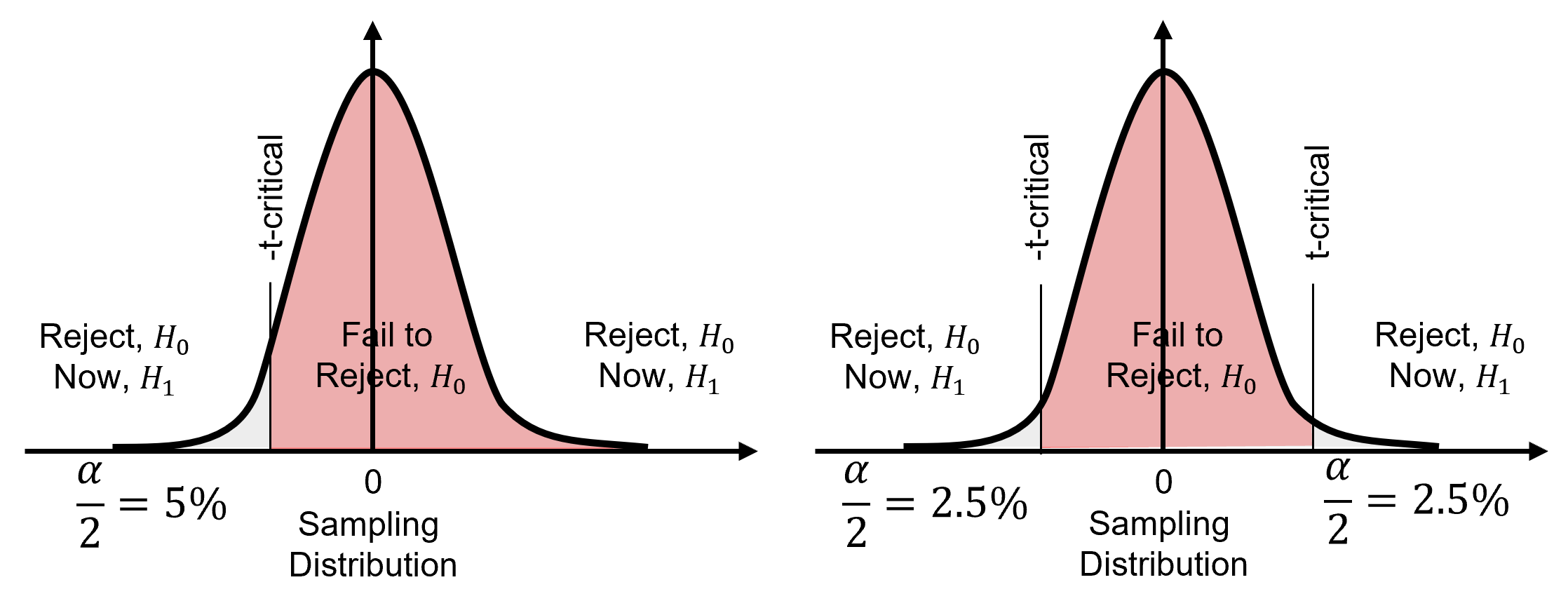
Here’s a one tail test, is well 1 in better rock than well 2 (by average porosity)? In this case we are only testing if well 1’s mean porosity is significantly greater than well 2’s mean porosity.
well 1 average porosity is less than or equal to the well 2 average porosity,
well 1 average porosity is greater than well 2 average porosity,
and now, here’s a two tail test, are wells 1 and 2 in different (according to average porosity)? In this case we are testing for significant difference without concern for which well has a larger mean.
well 1 & 2 average porosity are the same,
well 1 and 2 average porosity are the different,
The choice of one or two tail test also impacts the percentile applied. For a two tail test we split alpha over the lower and upper tails, so we use the percentile for,
while for a single tail test we order the measure so we only use the lower tail percentile for,
Limitations of Hypothesis Testing#
Before we go any further, let’s mention the limitations of hypothesis testing. This is really important, because these issues have caused hypothesis testing to fall out of favor in some scientific communities.
Publication Bias – only publish results that reject the null, i.e., show significant results
Recall, \(\alpha\) probability of false positive
Data mining for any effect will find insignificant differences that look significantly different (by random)
Meta studies have indicated the possibility that many studies have selectively reported significant results
Very small sample sizes, poorly understood phenomenon
we cannot demonstrate conformity with the test assumptions
Other Data Issues, Poor Sampling Practice
Contamination of sample, for example, the clever Hans effect where the examinee is taking cues from the examiner
Placebo effect, impact of subject motivation
Due to these there is some mistakes and skepticism concerning the use of hypothesis testing in publications. Solutions include avoiding small sample sizes and reporting p-values instead of binary reject or fail to reject
Pooled Variance Method for Difference in Means#
For the Student’s t-test, equal variances, pooled variance method (William Gosset, 1876-1937), we state the hypotheses as,
and then we use the Student’s t distribution to model the sampling distribution and calculate the t-statistic as,
where \(\bar{x}_1\) and \(\bar{x}_2\) are the sample means, \(s_1^2\) and \(s_2^2\) are the sample standard deviations, and \(n_1\) and \(n_2\) are the number of samples.
and then we calculate the \(t_{critical}\) as,
Then we fail to reject \(𝐻_0\) if,
or reject \(𝐻_0\) if,
Note, this test assumes that the variables are Gaussian distributed, and the standard deviations are not significantly different.
If your sample size is large enough, the central limit theorem suggests that the sampling distribution of the sample mean will approach normality, even if the data itself is not normally distributed.
In such cases, you may still use the t-test, but this assumes your sample sizes are sufficiently large (generally, n > 30 is considered acceptable).
Welch’s t-test for Difference in Means#
For the Student’s t-test for unequal variances, Welch’s t-test (Bernard Welch, 1911-1989), we again state the hypotheses as,
and then we use the Student’s t distribution to model the sampling distribution and calculate the t-statistic as,
where \(\bar{x}_1\) and \(\bar{x}_2\) are the sample means, \(s_1^2\) and \(s_2^2\) are the sample standard deviations, and \(n_1\) and \(n_2\) are the number of samples.
and then we calculate the \(t_{critical}\) as,
where \(\nu\) is calculated as,
and \(u\) is calculated as,
Then we fail to reject \(𝐻_0\) if,
or reject \(𝐻_0\) if,
Note, this test assumes that the variables are Gaussian distributed, and variances are unequal. Welch’s t-test.
If your sample size is large enough, the central limit theorem suggests that the sampling distribution of the sample mean will approach normality, even if the data itself is not normally distributed.
In such cases, you may still use the t-test, but this assumes your sample sizes are sufficiently large (generally, n > 30 is considered acceptable).
Demonstration of Difference Means Hypothesis Tests#
Example #1: Hypothesis Test for Difference in Means, Equal Variance Method
The samples include,
Well 1 - \(n_1 = 20\) samples, \(\bar{\phi_1} = 13%\), \(s_{\phi_1} = 2%\)
Well 2 - \(n_2 = 25\) samples, \(\bar{\phi_2} = 15%\), \(s_{\phi_2} = 3%\)
At a 95% confidence level (\(\alpha = 0.05\)) test \(𝐻_0: \mu_1= \mu_2\)
First we calculate the t-statistic, \(\hat{t}\), as,
we substitute and solve as,
Then we calculate the t-critical, \(t_{critical}\) as,
we substitute and solve as,
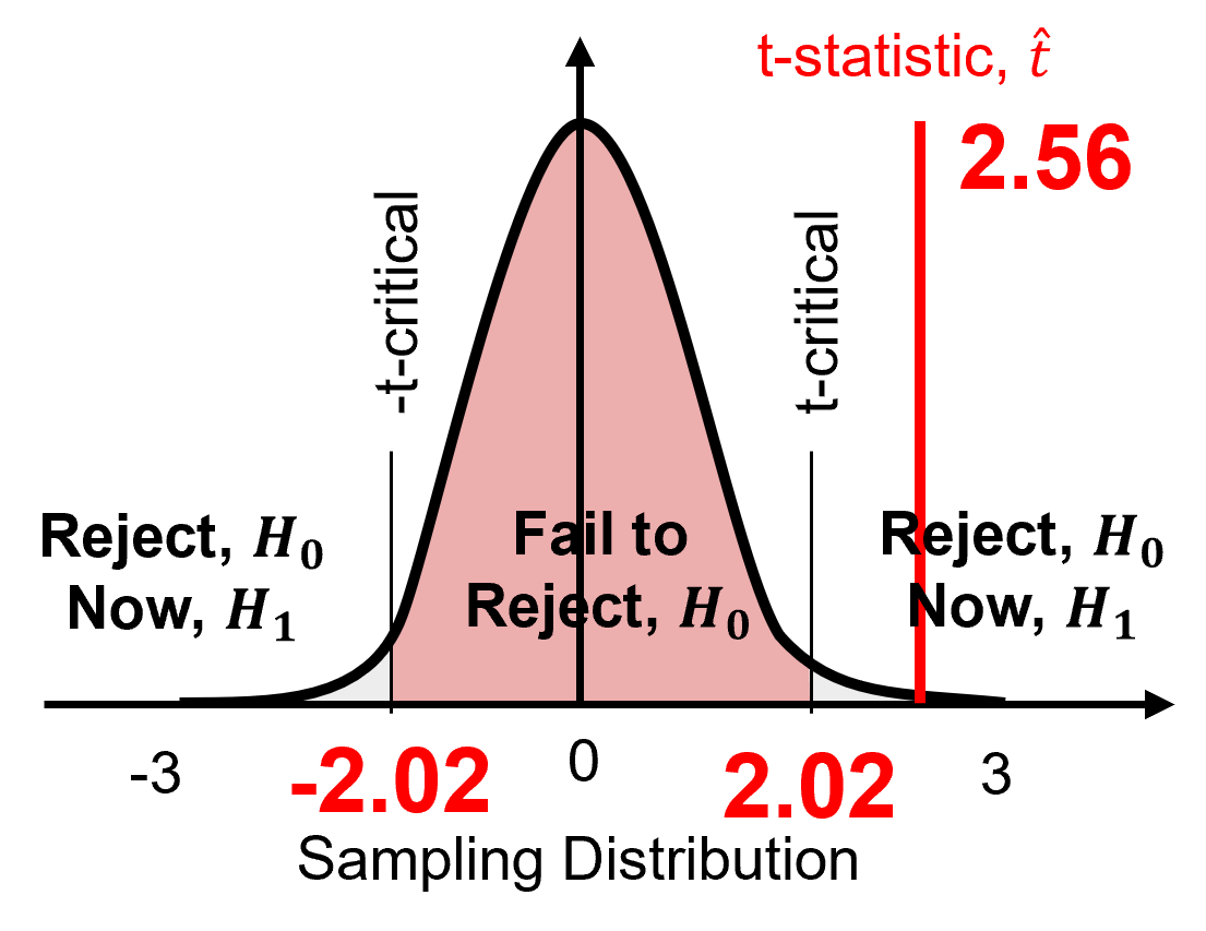
\(\hat{t} = 2.56\) is outside interval \([-2.02, 2.02]\) therefore, we reject the null hypothesis. We adopt the alternative hypothesis that,
If the means are significantly different, then the distributions are significantly different, and we are drilling potentially new rock.
F-test for Difference in Variances#
The F‐test for Difference in Variance (Snedecor and Cochran, 1989), we state the hypotheses as,
and then we use the F-distribution to model the sampling distribution and calculate the t-statistic as,
where \(s_1^2\) and \(s_2^2\) are the sample variances and then we calculate the \(F_{critical}\) as,
Then we reject \(𝐻_0\) if,
or fail to reject \(𝐻_0\) if,
Example #2: Hypothesis Test for Difference in Variances#
The samples include,
Well 1 - \(n_1 = 20\), \(s^2_{\phi_1} = 4%\)
Well 2 - \(n_2 = 25\), \(s^2_{\phi_2} = 9%\)
At a 95% confidence level (\(\alpha = 0.05\)) test \(\frac{\sigma_1^2}{\sigma_2^2} = 1.0\).
First we calculate the F-statistic, \(\hat{F}\), as,
we substitute and solve as,
Then we calculate the F-critical, \(F_{critical}\) as,
we substitute and solve as,
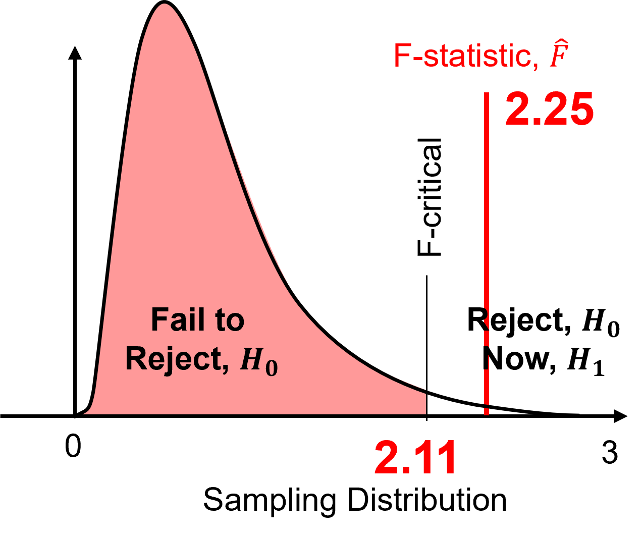
\(\hat{F} = 2.25\) is outside interval \([0, 2.11]\) therefore, we reject the null hypothesis. We adopt the alternative hypothesis that,
If the variances are significantly different, then the distributions are significantly different, and we are drilling potentially new rock.
Note, this test assumes the sample and population distributions are of both samples are Gaussian, but at 5% alpha with similar number of samples it is robust if non-normal (not Gaussian distributed).
Interactive Hypothesis Testing Dashboard#
To help visualize hypothesis testing, I built an interactive Python Hypothesis Testing Dashboard.
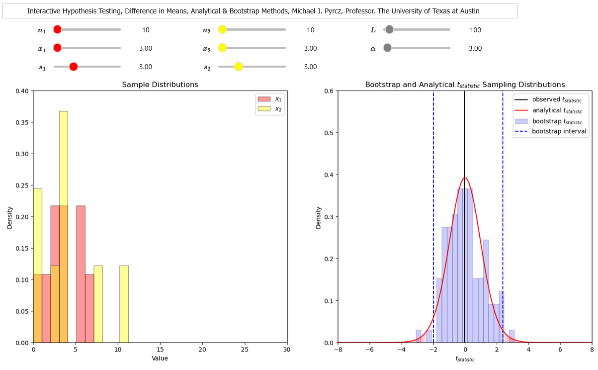
Now I demonstrate the following in Python,
Student-t hypothesis test for difference in means (pooled variance)
Student-t hypothesis test for difference in means (difference variances), Welch’s t Test
F-distribution hypothesis test for difference in variances
Load the Required Libraries#
The following code loads the required libraries.
import os                                                   # to set current working directory
import numpy as np                                          # arrays and matrix math
import scipy.stats as stats                                 # statistical methods
import pandas as pd                                         # DataFrames
import math                                                 # square root
import statistics                                           # statistics
import matplotlib.pyplot as plt                             # plotting
If you get a package import error, you may have to first install some of these packages. This can usually be accomplished by opening up a command window on Windows and then typing ‘python -m pip install [package-name]’. More assistance is available with the respective package docs.
Declare Functions#
def welch_dof(x,y):                                          # DOF for Welch's test from https://pythonfordatascienceorg.wordpress.com/welch-t-test-python-pandas/
        dof = (x.var()/x.size + y.var()/y.size)**2 / ((x.var()/x.size)**2 / (x.size-1) + (y.var()/y.size)**2 / (y.size-1))
        return dof
Set the working directory#
I always like to do this so I don’t lose files and to simplify subsequent read and writes (avoid including the full address each time). Also, in this case make sure to place the required (see below) data file in this directory. When we are done with this tutorial we will write our new dataset back to this directory.
#os.chdir("C:\PGE337") # set the working directory
Loading Data#
Let’s load the provided dataset. ‘PorositySamples2Units.csv’ is available at GeostatsGuy/GeoDataSets. It is a comma delimited file with 20 porosity measures from 2 rock units from the subsurface, porosity (as a fraction). We load it with the pandas ‘read_csv’ function into a data frame we called ‘df’ and then preview it by printing a slice and by utilizing the ‘head’ DataFrame member function (with a nice and clean format, see below).
df = pd.read_csv(r"https://raw.githubusercontent.com/GeostatsGuy/GeoDataSets/master/PorositySample2Units.csv") # load data from Prof. Pyrcz's github
df.head()                                                   # we could also use this command for a table preview
| X1 | X2 | |
|---|---|---|
| 0 | 0.21 | 0.20 |
| 1 | 0.17 | 0.26 |
| 2 | 0.15 | 0.20 |
| 3 | 0.20 | 0.19 |
| 4 | 0.19 | 0.13 |
It is useful to review the summary statistics of our loaded DataFrame. That can be accomplished with the ‘describe’ DataFrame member function. We transpose to switch the axes for ease of visualization.
df.describe().transpose() # statistical summaries
| count | mean | std | min | 25% | 50% | 75% | max | |
|---|---|---|---|---|---|---|---|---|
| X1 | 20.0 | 0.1645 | 0.027810 | 0.11 | 0.1500 | 0.17 | 0.19 | 0.21 |
| X2 | 20.0 | 0.2000 | 0.045422 | 0.11 | 0.1675 | 0.20 | 0.23 | 0.30 |
Here we extract the X1 and X2 unit porosity samples from the DataFrame into separate arrays called ‘X1’ and ‘X2’ for convenience.
X1 = df['X1'].values                                        # extract features as 1D ndarrays
X2 = df['X2'].values
Pooled Variance t-test Difference in Means#
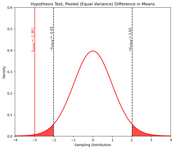
Now, let’s try the t-test, hypothesis test for difference in means. This test assumes that the variances are similar along with the data being Gaussian distributed (see the course notes for more on this). This is our test:
For the resulting t-statistic and p-value we run this command.
t_pooled, p_pooled = stats.ttest_ind(X1,X2)                 # assuming equal variance
print('The t statistic is ' + str(np.round(t_pooled,2)) + ' and the p-value is ' + str(np.round(p_pooled,5)))
The t statistic is -2.98 and the p-value is 0.00499
The p-value, \(p\), is the symmetric interval probability our outside.
In other words the \(p\) reported is 2 x cumulative probability of the t statistic applied to the sampling t distribution.
Another way to look at it, if one used the \(\pm t_{t_{statistic},.d.f}\) statistic as thresholds, \(p\) is the probability being outside this symmetric interval. So we will reject the null hypothesis if \(p \lt \alpha\).
From the p-value alone it is clear that we would reject the null hypothesis and accept the alternative hypothesis that the means are not equal.
In case you want to compare the t-statistic to t-critical, we can apply the inverse of the student’s t distribution at \(\frac{\alpha}{2}\) and \(1-\frac{\alpha}{2}\) to get the upper and lower critical values.
n1 = len(X1); n2 = len(X2)
smean1 = np.mean(X1); smean2 = np.mean(X2)
sstdev1 = np.std(X1); sstdev2 = np.std(X2,)
dof = len(X1)+len(X2)-2
t_critical = np.round(stats.t.ppf([0.025,0.975], df=dof),2)
print('The t critical lower and upper values are ' + str(np.round(t_critical,2)))
The t critical lower and upper values are [-2.02 2.02]
We can observe that, as expected, the t-statistic is outside the t-critical interval. These results are exactly what we got when we worked out the problem by hand in Excel, but so much more efficient!
Now, let’s plot this result.
xval = np.linspace(-4.0,4.0,1000)
tpdf = stats.t.pdf(xval,loc=0,df=dof,scale=1.0)
plt.plot(xval,tpdf,color='red',lw=2); plt.xlabel('Sampling Distribution'); plt.ylabel('Density')
plt.title('Hypothesis Test, Pooled (Equal Variance) Difference in Means')
plt.xlim([-4.0,4.0]); plt.ylim([0,0.6])

plt.annotate('$-t_{critical} = $' + str(t_critical[0]),[t_critical[0]-0.18,0.4],rotation=90.0)
plt.annotate('$+t_{critical} = $' + str(t_critical[1]),[t_critical[1]-0.18,0.4],rotation=90.0)
plt.annotate('$t_{pooled} = $' + str(np.round(t_pooled,3)),[t_pooled-0.18,0.4],rotation=90.0,color='red')

plt.fill_between(xval,tpdf,where= xval < t_critical[0], color='red',alpha=0.7)
plt.fill_between(xval,tpdf,where= xval > t_critical[1], color='red',alpha=0.7)
plt.vlines(t_critical,0,7,color='black',ls='--')
plt.vlines(t_pooled,0,0.7,color='red')

plt.subplots_adjust(left=0.0, bottom=0.0, right=1.0, top=1.1, wspace=0.3, hspace=0.4); plt.show()
Welch’s t-test Difference in Means#
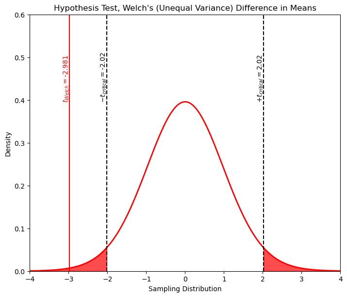
Now let’s try the t-test, hypothesis test for difference in means allowing for unequal variances, this is also known as the Welch’s t test, with the same hypotheses as above,
All we have to do is set the parameter ‘equal_var’ to false, note it defaults to true (e.g. the command above).
t_Welch,p_Welch = stats.ttest_ind(X1, X2, equal_var = False) # allowing for difference in variance
print('The t statistic is ' + str(np.round(t_Welch,2)) + ' and the p-value is ' + str(np.round(p_Welch,5)))
The t statistic is -2.98 and the p-value is 0.0055
Once again we can see by \(p\) that we will clearly reject the null hypothesis.
Now let’s plot the result,
xval = np.linspace(-4.0,4.0,1000)
tpdf = stats.t.pdf(xval,loc=0,df=welch_dof(X1,X2),scale=1.0)
plt.plot(xval,tpdf,color='red',lw=2); plt.xlabel('Sampling Distribution'); plt.ylabel('Density');
plt.title('Hypothesis Test, Welch\'s (Unequal Variance) Difference in Means')
plt.xlim([-4.0,4.0]); plt.ylim([0,0.6])

plt.annotate(r'$-t_{critical} = $' + str(t_critical[0]),[t_critical[0]-0.18,0.4],rotation=90.0)
plt.annotate(r'$+t_{critical} = $' + str(t_critical[1]),[t_critical[1]-0.18,0.4],rotation=90.0)
plt.annotate(r'$t_{Welch} = $' + str(np.round(t_Welch,3)),[t_Welch-0.18,0.4],rotation=90.0,color='red')

plt.fill_between(xval,tpdf,where= xval < t_critical[0], color='red',alpha=0.7)
plt.fill_between(xval,tpdf,where= xval > t_critical[1], color='red',alpha=0.7)
plt.vlines(t_critical,0,7,color='black',ls='--')
plt.vlines(t_pooled,0,0.7,color='red')

plt.subplots_adjust(left=0.0, bottom=0.0, right=1.0, top=1.1, wspace=0.3, hspace=0.4); plt.show()
F-test Difference in Variances#
Let’s now compare the variances with the F-test for difference in variances.
\begin{equation} H_0: \frac{\sigma^{2}{X_2}}{\sigma^{2}{X_1}} = 1.0 \end{equation}
\begin{equation} H_1: \frac{\sigma^{2}{X_2}}{\sigma^{2}{X_1}} > 1.0 \end{equation}
Note, by ordering the variances we eliminate the case of \(\sigma^{2}_{X_2} \lt \sigma^{2}_{X_1}\).
Details about the test are available in the course notes (along with assumptions such as Gaussian distributed) and this example is also worked out by hand in the linked Excel workbook. We can accomplish the F-test in with SciPy.Stats the function with one line of code if we calculate the ratio of the sample variances ensuring that the larger variance is in the numerator and get the degrees of freedom using the len() command, ensuring that we are consistent with the numerator degrees of freedom set as ‘dfn’ and the denominator degrees of freedom set as ‘dfd’. We take a p-value of \(1-p\) since the test is configured to be a single, right tailed test.
p_value = 1 - stats.f.cdf(np.var(X2)/np.var(X1), dfn=len(X2)-1, dfd=len(X1)-1)
p_value
0.019187348063153697
Once again we would clearly reject the null hypothesis since \(p \lt alpha\) and assume that the variances are not equal.
Compact Code Solution - Hypothesis Test, Student’s t-test for Difference in Means#
import numpy as np
import pandas as pd
import matplotlib.pyplot as plt
import scipy.stats as stats

df = pd.read_csv('https://raw.githubusercontent.com/GeostatsGuy/GeoDataSets/master/PorositySample2Units.csv')
X1 = df['X1'].values; X2 = df['X2'].values

alpha = 0.05
t_critical = stats.t.ppf(alpha/2,len(X1)+len(X2)-2)
t_pooled, p_pooled = stats.ttest_ind(X1,X2)                 # assuming equal variance
if(t_pooled < t_critical or t_pooled > -1*t_critical):
    print('Equal Variance: t-critical and t-statistic are ' + str(np.round(t_critical,2)) + ' ≤ ' + str(np.round(t_pooled,2)) +
      ' ≤ ' + str(np.round(-1*t_critical,2)) + '; therefore, reject the null hypothesis')
else:
    print('Equal Variance: t-critical and t-statistic are ' + str(np.round(t_critical,2)) + ' ≤ ' + str(np.round(t_pooled,2)) +
      ' ≤ ' + str(np.round(-1*t_critical,2)) + '; therefore, fail to reject the null hypothesis')

    alpha = 0.05
t_critical = stats.t.ppf(alpha/2,len(X1)+len(X2)-2)

t_welch, p_welch = stats.ttest_ind(X1,X2,equal_var = False) # assuming unequal variance, Welch's t-test
if(t_welch < t_critical or welch > -1*t_critical):
    print('Welch\'s test: t-critical and t-statistic are ' + str(np.round(t_critical,2)) + ' ≤ ' + str(np.round(t_welch,2)) +
      ' ≤ ' + str(np.round(-1*t_critical,2)) + '; therefore, reject the null hypothesis')
else:
    print('Welch\'s test: t-critical and t-statistic are ' + str(np.round(t_critical,2)) + ' ≤ ' + str(np.round(t_welch,2)) +
      ' ≤ ' + str(np.round(-1*t_critical,2)) + '; therefore, fail to reject the null hypothesis')
Equal Variance: t-critical and t-statistic are -2.02 ≤ -2.98 ≤ 2.02; therefore, reject the null hypothesis
Welch's test: t-critical and t-statistic are -2.02 ≤ -2.98 ≤ 2.02; therefore, reject the null hypothesis
Compact Code Solution - Hypothesis Test, F-test for Difference in Variances#
import numpy as np
import pandas as pd
import matplotlib.pyplot as plt
import scipy.stats as stats

df = pd.read_csv('https://raw.githubusercontent.com/GeostatsGuy/GeoDataSets/master/PorositySample2Units.csv')
X1 = df['X1'].values; X2 = df['X2'].values

alpha = 0.05
var_X1 = np.var(X1,ddof=1); var_X2 = np.var(X2,ddof=1)      # sample variance
f_stat = np.max([var_X1,var_X2])/np.min([var_X1,var_X2])
if var_X1 > var_X2:
    f_critical = stats.f.ppf(1-alpha,len(X1)-1,len(X2)-1)
else:
    f_critical = stats.f.ppf(1-alpha,len(X2)-1,len(X1)-1)
if f_stat > f_critical:
    print('f-statistic and f-critical are ' + str(np.round(f_stat,2)) + ' > ' + str(np.round(f_critical,2))
          + '; therefore, reject the null hypothesis')
else:
    print('f-statistic and f-critical are ' + str(np.round(f_stat,2)) + ' ≤ ' + str(np.round(f_critical,2))
          + '; therefore, fail to reject the null hypothesis')
f-statistic and f-critical are 2.67 > 2.17; therefore, reject the null hypothesis
About the Author#

Michael Pyrcz is a professor in the Cockrell School of Engineering, and the Jackson School of Geosciences, at The University of Texas at Austin, where he researches and teaches subsurface, spatial data analytics, geostatistics, and machine learning. Michael is also,
the principal investigator of the Energy Analytics freshmen research initiative and a core faculty in the Machine Learn Laboratory in the College of Natural Sciences, The University of Texas at Austin
an associate editor for Computers and Geosciences, and a board member for Mathematical Geosciences, the International Association for Mathematical Geosciences.
Michael has written over 70 peer-reviewed publications, a Python package for spatial data analytics, co-authored a textbook on spatial data analytics, Geostatistical Reservoir Modeling and author of two recently released e-books, Applied Geostatistics in Python: a Hands-on Guide with GeostatsPy and Applied Machine Learning in Python: a Hands-on Guide with Code.
All of Michael’s university lectures are available on his YouTube Channel with links to 100s of Python interactive dashboards and well-documented workflows in over 40 repositories on his GitHub account, to support any interested students and working professionals with evergreen content. To find out more about Michael’s work and shared educational resources visit his Website.
Want to Work Together?#
I hope this content is helpful to those that want to learn more about subsurface modeling, data analytics and machine learning. Students and working professionals are welcome to participate.
Want to invite me to visit your company for training, mentoring, project review, workflow design and / or consulting? I’d be happy to drop by and work with you!
Interested in partnering, supporting my graduate student research or my Subsurface Data Analytics and Machine Learning consortium (co-PI is Professor John Foster)? My research combines data analytics, stochastic modeling and machine learning theory with practice to develop novel methods and workflows to add value. We are solving challenging subsurface problems!
I can be reached at mpyrcz@austin.utexas.edu.
I’m always happy to discuss,
Michael
Michael Pyrcz, Ph.D., P.Eng. Professor, Cockrell School of Engineering and The Jackson School of Geosciences, The University of Texas at Austin
More Resources Available at: Twitter | GitHub | Website | GoogleScholar | Geostatistics Book | YouTube | Applied Geostats in Python e-book | Applied Machine Learning in Python e-book | LinkedIn
Comments#
I hope you found this chapter helpful. Much more could be done and discussed, I have many more resources. Check out my shared resource inventory,
Michael