Geostatistics Concepts

Geostatistics Concepts#

Michael J. Pyrcz, Professor, The University of Texas at Austin

Chapter of e-book “Applied Geostatistics in Python: a Hands-on Guide with GeostatsPy”.

Cite this e-Book as:

Pyrcz, M.J., 2024, Applied Geostatistics in Python: a Hands-on Guide with GeostatsPy, https://geostatsguy.github.io/GeostatsPyDemos_Book.

The workflows in this book and more are available here:

Cite the GeostatsPyDemos GitHub Repository as:

Pyrcz, M.J., 2024, GeostatsPyDemos: GeostatsPy Python Package for Spatial Data Analytics and Geostatistics Demonstration Workflows Repository (0.0.1). Zenodo. https://zenodo.org/doi/10.5281/zenodo.12667035

By Michael J. Pyrcz
© Copyright 2024.

This chapter is a summary of Geostatistics Concepts including essential concepts:

Statistics, Data Analytics, and Data Science
Geostatistics Prerequisite Definitions and Concepts
Guidance and Cautionary Statements

YouTube Lecture: check out my lecture on Data Analytics Concepts. For your convenience here’s a summary of salient points.

Motivation for Geostatistics Concepts#

You could just open up a Jupyter notebook in Python and start building spatial geostatistical models.

Alternatively, many “canned software” programs have geostatistics built in and often have reasonable default parameters to build spatial models.
There are many sources of code examples, including this e-book and my many well-documented Python workflows in my GeostatsPyDemos repository in my GitHub account that you could copy and paste and update for your own data.
Also, you could Google a question about using a specific geostatistical algorithm in Python and the top results may include StackOverflow questions and responses, it is truly amazing how much experienced coders are willing to give back and share their knowledge.

We truly have an amazing scientific community with the spirit of knowledge sharing and open-source development. Respect.

Of course, you could learn a lot about geostatistics from a machine learning large language model (LLM) like ChatGPT. Not only will ChatGPT answer your questions, but it will also provide codes and help you debug them when you tell ChatGPT what went wrong.

One way or the other you obtained and added this code to you data science workflow (taken from my [GeostatsPy_kriging] workflow at GeostatsGuy/GeostatsPyDemos),

por_vrange_maj2 = 150; por_vrange_min2 = 50                   # variogram ranges
por_vazi2 = 150.0                                             # variogram major direction
por_vrel_nugget2 = 0.0                                        # variogram nugget effect

por_vario2 = GSLIB.make_variogram(nug=por_vrel_nugget2*por_sill,nst=1,it1=1,cc1=(1.0-por_vrel_nugget2)*por_sill,
         azi1=por_vazi2,hmaj1=por_vrange_maj2,hmin1=por_vrange_min2) # porosity variogram

ktype = 0                                                     # kriging type, 0 - simple, 1 - ordinary
radius = 600                                                  # search radius for neighbouring data
nxdis = 1; nydis = 1                                          # number of grid discretizations for block kriging
ndmin = 0; ndmax = 10                                         # minimum and maximum data for an estimate

por_SK_kmap, por_vmap = geostats.kb2d(df,'X','Y','Porosity',pormin,pormax,nx,xmn,xsiz,ny,ymn,ysiz,nxdis,nydis,
         ndmin,ndmax,radius,0,por_skmean,por_vario2)

et voilà, you have a kriged map that could be applied to make predictions for new spatial samples and to assess resources, etc., and support some important development decision.

But, is this a good model? Did we do something wrong with the input parameters that we didn’t understand?
How good is it? Could it be improved?
Wait, should we actually use kriging for this problem? Or should we use simulation? Or maybe just a spreadsheet!

Without knowledge about basic geostatistics concepts we can’t answer these questions and build the best possible models. In general, I’m not an advocate for black box modeling, because it is:

likely to lead to mistakes that may be difficult to detect and correct
incompatible with the expectations for compentent practice for professional engineers. I gave a talk on Applying Machine Learning as a Compentent Engineer or Geoscientist
not fun to do. Do you remember those early days playing the guitar or participating in a martial art? Is it not more fun when we see our our personal growth and gain confidence in the things that we do?

To help you “look under the hood”, this chapter provides you with the basic knowledge to answer these questions and to make better, more reliable geostatistical models. Let’s start building this essential foundation with some general definitions.

Big Data#

Everyone hears that data science needs a lot of data. In fact, so much data that it is called “big data”, but how do you know if you are working with big data? The criteria for big data are these ‘V’s, if upon reflection you answer “yes” for at least some of these, then you are working with big data:

Volume: many data samples, difficult to handle and visualize
Velocity: high rate collection, continuous relative to decision making cycles
Variety: data form various sources, with various types and scales
Variability: data acquisition changes during the project
Veracity: data has various levels of accuracy

In my experience, most spatial and subsurface-focussed, engineers and (geo)scientists answer yes to all of these questions.

So I proudly say that we in space or specifically the subsurface have been big data long before the tech sector learned about big data.
In fact, I state that we in the subsurface resource industries are the original data scientists. I’m getting ahead of myself, more on this in a bit.

Don’t worry if I get carried away with hubris, rest assured this e-book is written for anyone interested to learn about geostatistics. You can skip the short sections on subsurface data science or read along if interested. Now that we know big data, let’s talk about the big topics.

Subsurface engineers and geoscientists:

work with big data and we are the original data scientists!

Statistics, Geostatistics and Data Analytics#

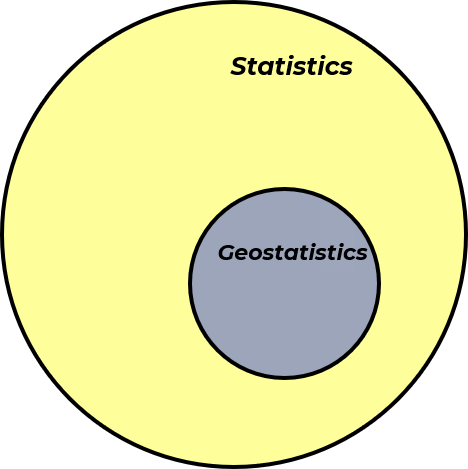
Statistics is collecting, organizing, and interpreting data, as well as drawing conclusions and making decisions. If you look up the definition of data analytics you will find criteria that include statistical analysis, and data visualization to support decision making. I’m going to call it, data analytics and statistics are the same thing.

Now we can append, geostatistics, as a branch of applied statistics that accounts for:

the spatial (geological) context
the spatial relationships
volumetric support
uncertainty

Remember all those statistics classes with the assumption of independent, identically distributed (remember the i.i.d.s everywhere?). Spatial phenomenon don’t do that, so we developed a unique branch of statistics to address this.

By our assumption above, we can state that geostatistics is the same as spatial data analytics.

Now, let’s use a Venn diagram to visualize statistics / data analytics and geostatistics / spatial data analytics:

Venn diagram for statistics and geostatistics.

Now we can add our previously discussed big data to our Venn diagram resulting in big data analytics and spatial big data analytics.

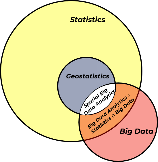
Venn diagram for statistics and geostatistics with big data added.

So, geostatistics is actually spatial data analytics, or more generally, let’s call it spatial data science. Now, let’s talk a bit about data science.

Data Science#

If no one else has said this to you, let me have the honor of welcoming you to the fourth paradigm for scientific discovery, data-driven scientific discovery or shortenned as data science.

The paradigms for scientific discovery are distinct stages or approaches for humanity to develop science.

To understand the fourth paradigm let’s compare to the previous three paradigms. Here’s all of the four paradigms with dates for important developments during each,

1st Paradigm Empirical Science	2nd Paradigm Theoretical Science	3rd Paradigm Computational Science	4th Paradigm Data Science
Experiments	Models and Laws	Numerical Simulation	Learning from Data
430 BC Empedocles proved air has substance	1011 AD al-Haytham Book of Optics	1942 Manhattan Project	2009 Hey et al. Data-Intensive Book
230 BC Eratosthenes measure Earth’s diameter	1687 AD Newton Principia	1980 – Global Forecast System (GFS)	2015 AlphaGo beats a professional Go player

Of course, we can argue about the boundaries between the paradigms for scientific discovery, i.e., when did a specific paradigm begin?

Certainly the Mesopotamians (4000 BC - 3500 BC) conducted many first paradigm experiments that supported their development of the wheel, plow, chariot, weaving loom, and irrigation and on the other side we can trace the development of artificial neural networks to McColloch and Pitts in 1943.
Also, the adoption of a new scientific paradigm is a major societal shift that does not occur uniformly around the globe.

So, what caused the fourth paradigm to start some time between 1943 and 2009? The fundamental mathematics of data driven models have been available for a long time, as demonstrated by the following mathematical and statistical developments in history,

Calculus - Isaac Newton and Gottfried Wilhelm Leibniz independently developed the math to find minimums and maximums during the 1600s with “Methods of Fluxions” 1671 (published posthumously in 1736), and with “Nova Methodus pro Maximis et Minimis” published in 1684.
Bayesian Probability - introduced by Reverend Thomas Bayes with Bayes’ Theorem enshrined in “An Essay Towards Solving a Problem in the Doctrine of Chances” published posthumously in 1763
Linear Regression - formalized by Marie Legendre in 1805
Discriminant Analysis - developed by Ronald Fisher in his 1939 paper “The Use of Multiple Measurements in Taxonomic Problems”
Monte Carlo Simulation - pioneered by Stanislaw Ulam and John von Neumann in the early 1940’s as part of the Manhattan Project

Upon reflection, one could ask, why didn’t the fourth paradigm start before the 1940’s and even in the 1800s? What changed? The answer is that other critical developments provided the fertile ground for data science, including cheap and available compute and big data.

Cheap and Available Compute#

Consider the following developments in computers,

Charles Babbage’s Analytical Engine (1837) is often credited as the first computer, yet is was a mechanical device the attempted to implement many modern concepts such as arithmetic logic, control flow and memory, but it was never completed given the challenges with the available technology.
Konrad Zuse’s Z3 (1941) and ENIAC (1945) the first digital, programmable computers, but they were programmed by labor-intensive and time-consuming rewiring of plug boards with machine language as there was no high level programming language, the memory could fit 1,000 words limiting the program complexity and with 1000s of vacuum tubes cooling and maintenance was a big challenge. These unreliable machines were very slow with only about 5,000 additions per second.
Transistors were invented in 1947 the transistor replaced the vacuum tubes greatly improving energy-efficiency, miniaturization, speed and reliability. Resulting in the second generation computers such as IBM 7090 and UNIVAC 1108.
Integrated Circuits were developed in the 1960s allowed for multiple transistors to be placed on a single chip leading to third generation computers.
Microprocessors - developed in 1971 integrated the functions of a computer’s central processing unit (CPU) enabling smaller, cheaper computers, resulting in the personal, home computer revolution including the Apple II (1977) and IBM PC (1981). Yes, when I was in grade 1 in elementary school we had a Apple II in my classroom, and it amazed all of us with the monochrome (orange and black pixels) monitor, floppy disk loaded programs (there was no hard drive) and beeps and clicks from the speaker!

We live in a society with more compute power in our pockets (cell phones) than used to send the first astronauts to the moon and a SETI screen saver that uses home computers’ idle time to search for extraterrestrial life! Now we are surrounded by cheap and reliable compute that our grandparents (and perhaps parents) could never have imagined.

As you will learn in this e-book, geostatistical methods requires a lot of compute.

In fact, calculating spatial models relies on a large number of iterations, matrix or parallel operations, bootstrapping models, stochastic descent over large grids often in the 10s - 100s of millions of cells, with several features at each cell, and uncertainty modeling requires a lot of scenarios and realizations.

Cheap and available compute is an essential prerequisite for the fourth paradigm. Now consider the development of data science has been largely a crowd-source, open-source effort. There cannot be data science without many people having easy access to compute.

Availability of Big Data#

With small data we tend to rely on other sources of information such as physics, engineering and geoscience principals and then calibrate these models to the few available observations, as is common in applications of the second and third paradigm for scientific discovery.

With big data we can learn the full range of behaviors of natural systems from the data itself.
In fact, with big data we often see the limitations of the second and third paradigm models due to missing complexity in our solutions.

Therefore, big data:

provides sufficient sampling to support the data-driven fourth paradigm
and may actually preclude exclusive use of the second and third paradigm

These days big data is everywhere, with so much data now open-source and available online. Here’s some great examples:

satellite data with time lapse is widely available on Google Earth and other platforms. Yes, this isn’t the most up to date and highest resolution statelite imagery, but it is certainly sufficient for many land use, geomorphology and surface evolution studies. My team of graduate students use it.
river gauges data over your state are generally available to the public. We use it for hydrologic analysis and also to determine great locations and times to paddle! Check out the USGS’s National Water Information System
government databases, including the United States Census to oil and gas production data are available to all
Moon Trek: online portal to visualize and download digital images from lunar orbiters, Lunar Reconnaissance Orbiter (LRO), SELENE and Clementine.

This is open, public data, but consider the fact that many industries are embracing smart, intelligent systems with enhanced connectivity, monitoring and control.

The result is an explosion of data supported by faster and cheaper computation, processing and storage.
We are all swimming in data that, once again, the generation before us could not have imagined.

Does anyone else go on Google Earth and explore new parts of our home planet? I have Google Earth for my HTC Vive Pro. I like to wander Skyrim, but often it is just as fun to explore our own Planet Earth in VR! So much data! We are so fortunate!

We could also talk about improved algorithms and hardware architectures optimized for data science, but I’ll leave that out of scope for this e-book.

All of these developments have provided the fertile ground for the seeds of spatial data science, geostatistics, to grow and become standard practice for management for the spatial and often the subsurface, including,

Mining developmental and critical minerals - in situ reosurces, development plan and reserves that maximize value and minimize environmental impact
Subsurface energy hydrocarbons, goethermal and hydrogen storage - in situ potential, development plan and reserves that maximize value and minimize environmental impact
Groundwater resources - model aquifer volume, recharge, discharge and drawdown, to support groundwater management, mitigation and policy.
Forestry - model forest inventory, corbon sequestration, to support silviculture.
Agriculture - modeling soils with digital elevation models to support precise agriculture to expand crop yeilds while protecting soil fertility and minimizing water and fertilizer use.

The world’s greatest problems

are spatial! Knowing spatial data science, geostatistics, is critical to take on these challenges.

Data Science and Subsurface Resources#

Spoiler alert, I’m going to boast a bit in the section. I often hear students say, “I can’t believe this data science course is in the Hildebrand Department of Petroleum and Geosystems Engineering!” or “Why are you teaching geostatistics in Department of Earth and Planetary Sciences?” My response is,

We in the subsurface are the original data scientists!

We are the original data-driven scientists, we have been big data long before tech learned about big data!

This may sound a bit arrogant, but let me back this up with this timeline:

Timeline of data science development from the perspective of subsurface engineering and geoscience.

Shortly after Kolmogorov developed the fundamental probability axioms during the 1930s,
Danie Krige developed a set of statistical, spatial, i.e., data-driven tools for making estimates in space while accounting for spatial continuity and scale in the 1950s.
These tools were formalized with theory developed by Professor Matheron during the 1960s in a new science called geostatistics.
Over the 1970s - 1990s the geostatistical methods and applications expanded from mining to address oil and gas, environmental, agriculture, fisheries, etc. with many important open source developments.

Why was subsurface engineering and geoscience earlier in the development of data science? Because, necessity is the mother of invention!

Complicated, heterogeneous, sparsely sampled, vast systems with complicated physics and high value decisions drove us to data-driven methods.

Contrast this with the many other engineering fields that:

work with homogeneous phenomenon that does not have significant spatial heterogeneity, continuity, nor uncertainty
have exhaustive sampling of the population relative to the modeling purpose and do not need an estimation model with uncertainty
have well understood physics and can model the entire system with second and third paradigm phenomenon

As a result, many of us subsurface engineers and geoscientists are applying and teaching spatial data science, geostatistics, and have been for many decades.

Population and Samples#

To understand geostatistics we need to first differentiate between the population and the sample, so that we can then understand the context for features, inference, prediction, etc.

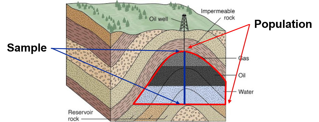
Population and sample (modified Image from https://energyeducation.ca/encyclopedia/Oil_and_gas_reservoir ).

Population - exhaustive, finite list of property of interest over area of interest. Generally the entire population is not accessible, e.g. exhaustive set of porosity at each location within a gas reservoir. To give you a sense of the vast scale of populations, consider these two examples:

Bingham Canyon Mine (also known as Kennecott Copper Mine) is a porphyry copper deposit in Utah, USA. The open pit is the largest anthropogenic excavation by volume extracted (6.5 \(m^3\)), and at 1,200 m deep, the deepest open pit mine in the world. The geology includes multiple zones of mineralization (magnitite central core zone, moybdenite zone, bornite-chalcopyrite-gold zone, pyrite-clacopyrite zone, pyrite zone and outermost lead-zinc zone with Late Paleozoic formations thrust faulted over Precambian craton. The features of interest include zonation (see above), grade shells (high, low, waste) with soft and hard boundaries, ore grades (copper, silver, gold, molybdenum, platinum and palladium) and contaminants (arsenic, lead, sulfur, etc.) (Wikipedia Bingham Canyon Mine).
Plutonio Reservoir, from the passive continential margin, Lower Congo Basin, Angola is a deepwater channel complex over a large volume of interest (6 km x 9 km x 120 m) (Oligocene O73 layer only), including distinct channel-related elements (inner channel, outer channel and overbank) with distinct porosity and permeability distributions. The features of interest include elements, porosity and permeability, represented in a model at 50 m x 50 m x 1 m resolution (2,556,120 cells) and conditioned by sparse near vertical wells (600 - 800 m spacing) and secondary feature, seismic RMS amplitude that is correlated with porosity and allows the channel complex and some channel elements to be mapable (Yanshu et al., 2020) {cite}`yanshu2020’

Sample - the set of measurements for the features of interest at locations that have been measured, e.g. porosity data from well-logs within a reservoir. Yet, there is more, for every sample we are concerned with,

what is the support volume of the sample’s measurement, i.e., over what volume have we measured?
what does the measurement tell us? All measurements must have a line-of-sight to value. E.g., porosity relates to volumetrics, and facies are useful for mapping porosity away from wells, etc.
what is the accuracy of the measurement? I’m sorry, but none of our subsurface measurements are certain. They all have measurement and interpretation errors.
what is the metadata related to the data? In the subsurface we have a lot of metadata, e.g., what were the assumptions made to calculate the measure? In the subsurface, all of our measure require interpretation (see an example below).

What are we measuring in our samples? Each distinct type of measure is called a variable or feature.

Variable or Feature#

Variable or Feature - any property measured / observed in a study, and in data science only the term feature is used. Note, all of us old school statisticians we are more accustomed with the term “variable”, but it is the same. Here’s some examples of features:

porosity measured from 1.5 inch diameter, 2 inch long core plugs extracted from the Miocene-aged Tahiti field in the Gulf of Mexico
permeability modeled from porosity (neutron density well log) and rock facies (interpreted fraction of shale logs) at 0.5 foot resolution along the well bore in the Late Devonian Leduc formation in the Western Canadian Sedimentary Basin.
blast hole cuttings derived nickel grade aggregated over 8 inch diameter 10 meter blast holes at Voisey’s Bay Mine, Proterozoic gneissic complex.

Did you see what I did? To describe features, I specified,

what was measured, how it was measured, and over what scale was it measured.

This is important because,

how the measure is made changes the veracity (level of certainty in the measure) and different methods actually may results in different results so we may need to reconcile multiple measurement methods of the same thing, so we often store each vintage as separate features.
the scale of the measure is very important due to volume variance effect, with increasing support volume (sample size) the variance reduces due to volumetric averaging resulting in regression to the mean. I have a chapter on volume-variance in my Applied Geostatistics in Python e-book for those interested in more details.

Additionally, our subsurface measures often requires significant analysis, interpretation, etc.

We don’t just hold a tool up to the rock and get the number, we have a thick layer of engineering and geoscience interpretation to map from measurement to a useable feature.

Consider this carbonate thin section from Bureau of Economic Geology, The University of Texas at Austin from geoscience course by F. Jerry Lucia.

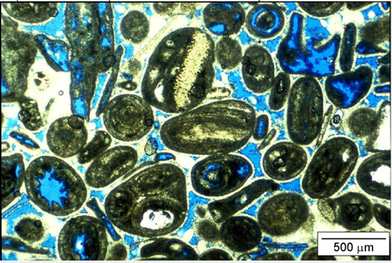
Carbonate thin section image (from this link by F. Jerry Lucia).

Note, the blue dye indicates the void space in the rock, but is porosity the blue area divided by the total area of the sample?

That would be the “total porosity” and not all of it may contribute to fluid flow in the rock as it is not sufficiently connected; therefore, we need to go from total porosity to “effective porosity”, requiring interpretation.

Even porosity, one of the most simple (observable in well logs and linearly averaging) features doesn’t escape essential interpretation.

Predictor and Response Features#

To understand the difference between predictor and response features let’s look at the most concise, simple expression of a data science model.

The fundamental predictive machine learning model that maps from predictor to response features.

The predictors (or independent) features (or variables) the model inputs, i.e., the \(X_1,\ldots,X_m\), response (or dependent) feature(s) (or variable(s)) are the model output, \(y\), and there is an error term, \(\epsilon\).

Data science is all about estimating such models, \(\hat{𝑓}\), for two purposes, inference or prediction.

Inference and Prediction#

Inference must precede prediction, because inference is going from the limited sample to a model of the population. Inference is learning about the system, \(\hat{f}\), for example,

what is the relationship between the features?
what feature are most important?
what are the complicated interactions between all the features?

A good example of a inferential problem is imagine if I walk in the room and pull a coin out of my pocket and flip it 10 times and get 3 heads and 7 tails and then ask you, “Is this is a fair coin?”.

you take the sample, the results from 10 coin tosses, to make an inference about the population, i.e., whether the coin is fair or not? Note, in this example the coin is the population!

Once we have completed our inference to model the population from the sample, we are ready to use the model of the population to predict future samples. This is prediction, going from a model of the population to estimating new samples.

the goal of prediction is to get the most accurate estimates of future samples.

Carrying on with our coin example, if you declare that my coin was biased towards tails (a weighted coin would be a useful teaching tool!) with a 70% probability of tails, now you are able to predict the outcome for the next 10 coin tosses, even before I toss the coin again. This is prediction.

How do you know if you are doing inferential or predictive machine learning. In general, inferential machine learning is conducted only with the predictor features, also known as unsupervised machine learning (because there are no response labels). Examples includes:

cluster analysis - that learns ways to split the data into multiple distinct populations to improve the subsequent models
dimensionality reduction - that projects the predictor features to a reduced number of new features that better describe the system with less noise

When you’re doing predictive machine learning you have both the predictor and the response feature(s), so we call it supervised learning. The model is trained and tuned to predict new samples.

Inference is going from a sample to a model of the population. Prediction is going from a model of the population to a prediction of the next sample. Inference preceeds prediction.

Determinstic vs. Stochastic Modeling#

Determinstic Model - A model based on a mathematical algorithm that produces the same output each time it is used with the same input. For example, an interpolation method and a numerical physics-based flow simulation are both deterministic models, because if we rerun them for a specific case, the answer does not change.

Consider these examples:

a best fit trend line, e.g., linear regression
regression tree
support vector machines

These are all determinsitic models. But, for geostatistics there is an important difference in how we see deterministic model. Let’s emphasize it here.

Deterministic Models Definition:

A model that provides a single best estimate and does not attempt to provide a model of uncertainty.

In geostatistics, we define deterministic modeling is any model that ignores uncertainty! Now we can add another type of models that may not be completely repeatable, but does not integrate uncertainty, models based on expert interpretation. Now imagine experts crafting the model and we can conceive of these advantages and disadvantages for the deterministic modeling approach,

Advantages of deterministic models:

integration of physics and expert knowledge - physics
integration of various information sources

Disadvantages of deterministic models:

often quite time consuming
often no assessment of uncertainty, focus on building one model

Stochastic Model - A model based on a probablistic model and random process that produces a new model every time it is run, usually by changing the random number seed. These models often focus on the statistical descriptions from the data at the expense of expert interpretation and physics, but are often faster and provide uncertainty models through multiple realizations.

Advantages of stochastic models:

speed, much faster than interpretation workflows
uncertainty assessment through realizations
report significance, confidence / prediction intervals
honor many types of data, often by encoding various data sources as probablities and combining them, e.g., Bayesian updating
data-driven approach that may be seen as more objective than expert-based
paradoxically more repeatable, given the same random number seed vs. deterministic models based on interpretation

Disadvantages of stochastic models:

no physics or limited physics integrated through trend models
statistical model assumptions and simplification that may limit the ability to model complicated natural phenomenon

Spoiler alert, geostatistics includes deterministic and stochastic spatial modeling methods, for example, inverse distance is deterministic and sequential Gaussian simulation is stochastic.

Kriging is interesting, because it provides a single best estimate that doesn’t change when we rerun it (no random number seed is applied), but it also provides a measure of uncertainty through the kriging estimation variance.
Let’s still call kriging a deterministic model

Hybrid Modeling - most subsurface models include a combination of determinstic and stochastic modeling. For example, a deterministic trend model based on interpretation may be applied to calculate a residual feature that is then modelled stochastically.

Hybrid modeling is more common than strictly stochastic modeling for spatial, subsurface resources.

Now we can clarify this discussion by including the specific modes of spatial, subsurface modeling.

Estimation vs. Simulation#

Now we can differentiate estimation and simulation. The act calculating the single best estimate of a feature over location(s) in space is spatial estimation. Let’s concisely summarize:

Estimation has these characteristics,

is process of obtaining the single best value of a subsurface feature at an unsampled location
local accuracy takes precedence over global spatial variability
too ‘smooth’, not appropriate for forecasting

In contrast, the act of calculating a set of good realizations of a feature over location(s) in space is spatial simulation.

Simulation has these characteristics,

is process of obtaining one or more good values of a reservoir property at an unsampled location
global accuracy, matches the global statistics
simulation methods tend to produce more realistic feature spatial, univariate distributions

Now we can connect this with the previous discussion,

deterministic models estimate, while stochastic models simulate

How do we choose between estimation and simulation? When would we prefer simulation over estimation?

we need to reproduce the distributions of features of interest, i.e., the extreme values matter
we need realistic spatial heterogeneity models for flow simulation

Subsurface Uncertainty Modeling#

What is uncertainty modeling? To answer this question, we need to back up and ask a more fundamental question, what is subsurface uncertainty? Let’s describe the concepts of subsurface uncertainty.

Uncertainty is not an intrinsic property of the subsurface.

At every location (\(\bf{u}_{\alpha}\)) within the volume of interest the features’ values (e.g., facies, porosity etc.) could be measured if we had access. Uncertainty is a function of our ignorance, our inability to observed and measure the subsurface with the coverage and scale required to support our scientific questions and decision making.

This sparsity of sample data combined with heterogeneity results in uncertainty.

If the subsurface was homogeneous then with few measurements uncertainty would be reduced and estimates resolved to a sufficient degree of exactitude.

Subsurface uncertainty is a model. We should use the term “uncertainty model”.

As with all models, our uncertainty model is imperfect, but useful.
Our uncertainty assessment is a function of a set of subjective decisions and parameter choices.
The degree of objectivity is improved by ensuring each of the decisions and parameters are defendable given the available data and judicious use of analogs.

Subsurface Uncertainty Definition:

Uncertainty is a function of our ignorance, our inability to observed and measure the subsurface with the coverage and scale required to support our scientific questions and decision making.

How Do We Represent Uncertainty? With uncertainty models built on the concept of random variables and random functions.

Random Variables - a random variable is a property at a location (\(\bf{u}_{\alpha}\)) that can take on multiple possible outcomes. This is represented by a probability density function (PDF).
Random Functions - if we take a set of random variables at all locations of interest and we impart the correct spatial continuity between them then we have a random function. Each outcome from the random function is a potential model of the subsurface.
Using Multiple Models - we represent uncertainty with multiple models. It is convenient to assume that each model is equiprobable, but one could assign variable probability based on available local information and analogs.
Realizations - multiple models to represent uncertainty where the input decisions and parameters are held constant and only the random number seed is changed to represent spatial away from data uncertainty.
Scenarios - multiple models to represent uncertainty where the input decisions and parameters are changed to represent model decision and input uncertainty.

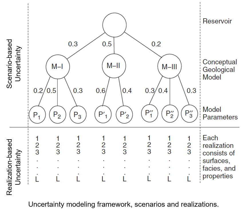
Uncertainty modeling with scenarios with different model parameters and choices and realizations with constant model parameters and choices, but with variable random number seed (from Pyrcz and Deutsch, 2014).

Working With Multiple Models: It is generally not appropriate to analyze a single or few scenarios and realizations. As Deutsch has taught during the 2017 IAMG lecture tour, for decision making, use all the models (realizations) all the time applied to the transfer function (e.g. volumetric calculation, contaminant transport, ore grade scale up, flow simulation etc.).

There is so much more that we could discuss about uncertainty modeling, for brevity I’ll just provide these additional points:

Calculating Uncertainty in a Modeling Parameter - use Bayesian methods, spatial bootstrap, etc. You must account for the volume of interest, sample data quantity and locations, and spatial continuity.
If You Know It, Put It In - use expert geologic knowledge and data to model trends. Any variability captured in a trend model is known and is removed from the unknown, uncertain component of the model. Overfit trend will result in unrealistic certainty.
Types of Uncertainty - include, (1) data measurement, calibration uncertainty, (2) modeling scenarios, decisions and parameters uncertainty, and (3) spatial uncertainty in estimating away from data. Your job is to hunt for and include all significant sources of uncertainty. I know there is more formal nomenclature for uncertainty sources, but I prefer these descriptive terms for teaching.
What about Uncertainty in the Uncertainty? Don’t go there. Use defendable choices in your uncertainty model, be conservative about what you known, document and move on. Matheron taught us to strip all away all defenseless assumptions. Journel warned us to avoid the circular quest of uncertainty in uncertainty in…
Uncertainty Depends on Scale - it is much harder to predict a property of teaspoon vs. a house-sized volume at a location (uα) in the subsurface. Ensure that scale and heterogeneity are integrated.
You Cannot Hide From It - ignoring uncertainty assumes certainty and is often a very extreme and dangerous assumption.
Decision Making with Uncertainty - apply all the models to the transfer function to calculate uncertainty in subsurface outcome to support decision making in the presence of uncertainty.
Uncertainty is a model - there is no objective uncertainty. Remember to always say, uncertainty model, not just uncertainty, to reflect this.
In general, increasing data sampling paucity, measurement error and bias, and level of heterogeneity all increase uncertainty.

Now we are ready to put it all together with the common geostatistical modeling workflow.

The Common Geostatistical Modeling Workflow#

While geostatistical modeling workflows are diverse and fit-for-purpose, this is the common workflow’s essential steps:

Integrate all available information to build multiple scenarios and realizations to sample the uncertainty space
Apply all the models to the transfer function to map to a decision criteria
Assemble the distribution of the decision criteria
Make the optimum decision accounting for this uncertainty model

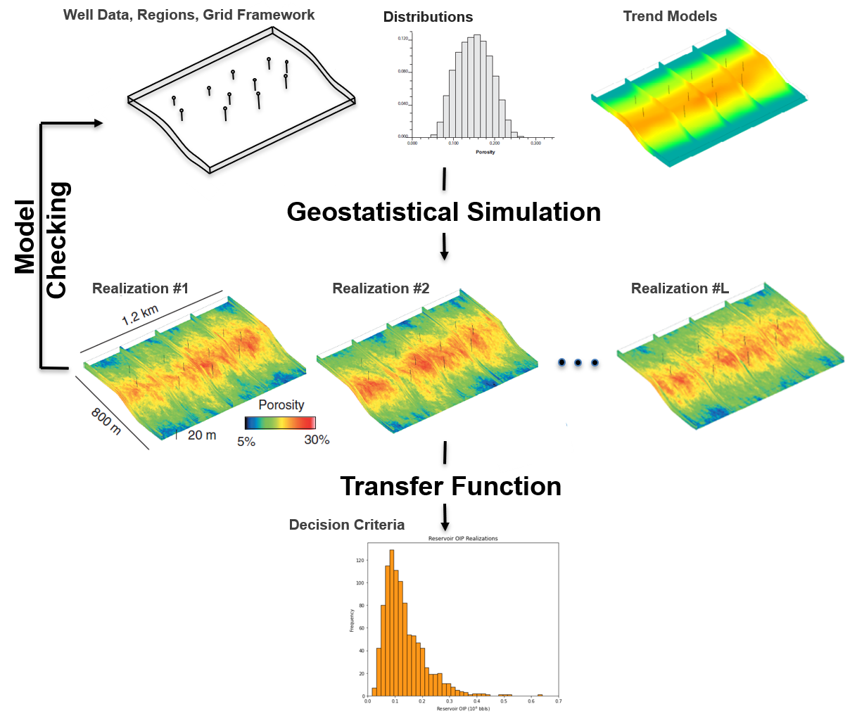
The common geostatistical modeling workflow (modified from Pyrcz and Deutsch, 2014).

Let’s fill in the one gap here, what is the?

Transfer Function - a operation that maps the models to the decision criteria, a measure of value! For example,

the transfer function could be a volumetric calculation to map models to total gold in place, e.g., 25 million ounces of gold, or
the transfer function could be a more complicated numerical simulation (3rd paradigm) to calculate total produced gas in 10 years, e.g., 11,000 Bcf.

As a data science-based approach, geostatistics has various ethical and professional practice concerns.

Teaching and Using Statistics and Data Analytics#

I encounter many professional engineers and scientists that are hessitant to use statistics and data analytics. The words of Hadley Wickham, Chief Scientist at Posit (the developers of RStudio) help me understand the potential cause of this hessitancy with his excellent short paper on the teaching statistics titled, Teaching Safe-Stats, Not Statistical Anstinence.

From my interpretation of Hadley’s paper, I summarize the following issues:

statistical perfectionism, we focus too much on doing exactly the write thing, rather than doing something useful.
stigmatize amateur statistics, we teach statistics should only be applied by the elite domain experts and not skilled practitioners.

Hadley’s solutions to these issues, to enable a greater level of statistical adoption in our engineering and scientific communities include,

develop statistical tools that are safer. This is one of the reasons that I love working with R, the packages are very well-documented, and with a single function you not only complete the statistical step, but you also get the diagnostic plots and summaries for safer, guided statistical tool use.
development of grammars of data analytics, frameworks for the minimal set of independent components and the methods to combine them to build workflows. This grammar approach is balanced for flexibility to adapt exisiting workflows and append new steps to take on new challenges. Constraints are included to prevent common mistakes or warn of potential mistakes.

Ethical and Professional Practice Concerns with Data Science#

Allow me to finish this discussion with a cautionary note. Rideiro et al. (2016) trained a logistic regression classifier with 20 wolf and dog images to detect the difference between wolves and dogs.

The input is a photo of a dog or wolf and the output is the probability of dog and the compliment, the probability of wolf.

The model worked well until this example here (see the left side below),

Example dog misclassified as a wolf (left) and pixels that resulted in this misclassification (right), image taken from Rideiro et al. (2016).

where this results in a high probability of wolf. Fortunately the authors were able to interrogate the model and determine the pixels that had the greatest influence of the model’s determination of wolf (see the right side above). What happened?

They trained a model to check for snow in the background.

As a Canadian I can assure you that many photos of wolves are in our snow filled northern regions of our country, while many dogs are photographed in grassy yards. The problem with machine learning is:

interpretability may be low with complicated models
application of machine learning may become routine and trusted

This is a dangerous combination, as the machine may become a trusted unquestioned authority. Rideiro and others state that they developed the problem to demonstrate this, but does it actually happen? Yes.

I advised a team of students that attempted to automatically segment urban vs. rural environments from time lapse satellite photographs to build models of urban development.
The model looked great, but I asked for an additional check with a plot of the by-pixel classification vs. pixel color. The results was a 100% correspondence, i.e., the model with all of it’s complicated convolution, activation, pooling was only looking for grey and tan pixels often associated with roads and buildings.

I’m not going to say, ‘Skynet’, oops I just did, but just reflect on my concerns with the broad use of data science:

Non-scientific results such as Clever Hans effect with models that learn from tells in the data rather than really learning to perform the task resulting catastrophic failures
New power and distribution of wealth and control by concentrating rapid inference with big data as more data is being shared
Model trade-offs that matter to society while maximizing a data science objective function may be ignored or poorly understood
Complicated data science models may become routine and may have low interpretability, resulting in unquestioned authority for the models
Societal changes and disruptive technologies, I am quite concerned about the unanticipated consequences of a post-labor society

I don’t want to be too negative and to take this discussion too far. I am a fan of science fiction and space futurism and I could definitely continue. I’ve thought about writing a fiction one day.

Full disclosure, I’m the old-fashioned professor that thinks we should put of phones in our pockets, walk around with our heads up so we can greet each other and observe our amazing environments and societies. One thing that is certain, data science is changing society in so many ways and as Neil Postman in Technopoly)

Neil Postman’s Quote for Technopoly

“Once a technology is admitted, it plays out its hand.”

Like-wise, geostatistics is a data sicence technology and it can be dangerous. Applied as a black-box it is a method to rapidly calculate realistic-appearing models, but,

Heterogeneity and stochasticity of geostatistical models may hide issues with the models.
The reliance on data-driven approaches motivate individuals to skip critical data and model checking and interpretation steps based on domain expertise.

Remember, 90% of our spatial data science projects is data preparation! We need to adhere to professional practice standards and have domain expertise for competent practice.

Comments#

This was a basic introduction to geostatistics. If you would like more on these fundamental concepts I recommend the Introduction, Modeling Principles and Modeling Prerequisites chapters from my text book, Geostatistical Reservoir Modeling{cite}`pyrcz2014’.

I hope this is helpful,

Michael

The Author:#

Michael Pyrcz, Professor, The University of Texas at Austin Novel Data Analytics, Geostatistics and Machine Learning Subsurface Solutions

With over 17 years of experience in subsurface consulting, research and development, Michael has returned to academia driven by his passion for teaching and enthusiasm for enhancing engineers’ and geoscientists’ impact in subsurface resource development.

For more about Michael check out these links:

Want to Work Together?#

I hope this content is helpful to those that want to learn more about subsurface modeling, data analytics and machine learning. Students and working professionals are welcome to participate.

Want to invite me to visit your company for training, mentoring, project review, workflow design and / or consulting? I’d be happy to drop by and work with you!
Interested in partnering, supporting my graduate student research or my Subsurface Data Analytics and Machine Learning consortium (co-PIs including Profs. Foster, Torres-Verdin and van Oort)? My research combines data analytics, stochastic modeling and machine learning theory with practice to develop novel methods and workflows to add value. We are solving challenging subsurface problems!
I can be reached at mpyrcz@austin.utexas.edu.

I’m always happy to discuss,