

Variogram Models, Simulation Examples#
Michael J. Pyrcz, Professor, The University of Texas at Austin
Twitter | GitHub | Website | GoogleScholar | Book | YouTube | Applied Geostats in Python e-book | LinkedIn
Chapter of e-book “Applied Geostatistics in Python: a Hands-on Guide with GeostatsPy”.
Cite this e-Book as:
Pyrcz, M.J., 2024, Applied Geostatistics in Python: a Hands-on Guide with GeostatsPy [e-book]. Zenodo. doi:10.5281/zenodo.15169133 ![]()
The workflows in this book and more are available here:
Cite the GeostatsPyDemos GitHub Repository as:
Pyrcz, M.J., 2024, GeostatsPyDemos: GeostatsPy Python Package for Spatial Data Analytics and Geostatistics Demonstration Workflows Repository (0.0.1) [Software]. Zenodo. doi:10.5281/zenodo.12667036. GitHub Repository: GeostatsGuy/GeostatsPyDemos ![]()
By Michael J. Pyrcz
© Copyright 2024.
This chapter is a tutorial for / demonstration of Visualizing Variogram Models in 1D Simulation with GeostatsPy.
YouTube Lecture: check out my lectures on:
Stochastic Simulation. For your convenience here’s a summary of salient points.
Variogram Modeling#
Spatial continuity can be modeled with nested, positive definite variogram structures:
where \(\Gamma_x(\bf{h})\) is the nested variogram model resulting from the summation of \(nst\) nested variograms \(\gamma_i(\bf{h})\).
The types of structure commonly applied include:
spherical
exponential
Gaussian
nugget
Other less common models include:
hole effect
dampened hole effect
power law
these will not be covered here.
Each one of these variogram structures, \(\gamma_i(\bf{h})\), is based on a geometric anisotropy model parameterized by the orientation and range in the major and minor directions. In 2D this is simply an azimuth and ranges, \(azi\), \(a_{maj}\) and \(a_{min}\). Note, the range in the minor direction (orthogonal to the major direction).
The geometric anisotropy model assumes that the range in all off-diagonal directions is based on an ellipse with the major and minor axes aligned with and set to the major and minor for the variogram.
Therefore, if we know the major direction, range in major and minor directions, we may completely describe each nested component of the complete spatial continuity of the variable of interest, \(i = 1,\dots,nst\).
Some comments on modeling nested variograms:
we can capture nugget, short and long range continuity structures
we rely on the geometric anisotropy model, so all structures must inform the same level of contribution (proportion of the sill) in all directions.
the geometric anisotropy model is based on azimuth of the major direction of continuity, range in the major direction and range in the minor direction (orthogonal to the major direction). The range is interpolated between the major and minor azimuths with a ellipse model
we can vary the type of variogram, direction or azimuth of the major direction, and major and minor ranges by structure
Sequential Gaussian Simulation#
With sequential Gaussian simulation we build on kriging by:
adding a random residual with the missing variance
sequentially adding the simulated values as data to correct the covariance between the simulated values
The resulting model corrects the issues of kriging, as we now:
reproduce the global feature PDF / CDF
reproduce the global variogram
while providing a model of uncertainty through multiple realizations
To help calibrate your eye, I provide examples of 1D simulated realizations with their associated variogram models.
Load the Required Libraries#
The following code loads the required libraries.
import geostatspy.GSLIB as GSLIB                              # GSLIB utilities, visualization and wrapper
import geostatspy.geostats as geostats                        # GSLIB methods convert to Python
import geostatspy
print('GeostatsPy version: ' + str(geostatspy.__version__))
GeostatsPy version: 0.0.71
We will also need some standard packages. These should have been installed with Anaconda 3.
import os                                                     # set working directory, run executables

from tqdm import tqdm                                         # suppress the status bar
from functools import partialmethod
tqdm.__init__ = partialmethod(tqdm.__init__, disable=True)

ignore_warnings = True                                        # ignore warnings?
import numpy as np                                            # ndarrays for gridded data
import pandas as pd                                           # DataFrames for tabular data
import matplotlib.pyplot as plt                               # for plotting
from matplotlib.ticker import (MultipleLocator, AutoMinorLocator) # control of axes ticks
from matplotlib import gridspec                               # customized subplots
from scipy import stats                                       # summary statistics
import math                                                   # trig etc.
import scipy.signal as signal                                 # kernel for moving window calculation
import random
plt.rc('axes', axisbelow=True)                                # plot all grids below the plot elements
if ignore_warnings == True:
    import warnings
    warnings.filterwarnings('ignore')
cmap = plt.cm.inferno                                         # color map
from IPython.utils import io                                  # mute simulation outputs
If you get a package import error, you may have to first install some of these packages. This can usually be accomplished by opening up a command window on Windows and then typing ‘python -m pip install [package-name]’. More assistance is available with the respective package docs.
Declare Functions#
This is a convenience function to add major and minor gridlines to our plots.
def add_grid():
    plt.gca().grid(True, which='major',linewidth = 1.0); plt.gca().grid(True, which='minor',linewidth = 0.2) # add y grids
    plt.gca().tick_params(which='major',length=7); plt.gca().tick_params(which='minor', length=4)
    plt.gca().xaxis.set_minor_locator(AutoMinorLocator()); plt.gca().yaxis.set_minor_locator(AutoMinorLocator()) # turn on minor ticks
Make a Simple Dataset#
We build a reference distribution, data outside the model to control the distribution only.
Then we add 3 points along a 1D section.
df = pd.DataFrame(np.vstack([np.full(1000,-9999),np.random.normal(size=1000),
                np.random.normal(loc=1000,scale=200,size=1000)]).T, columns= ['X','Y','Lithium'])
df.loc[0,'X'] = 105; df.loc[0,'Y'] = 5.0; df.loc[0,'Lithium'] = 800
df.loc[1,'X'] = 505; df.loc[1,'Y'] = 5.0; df.loc[1,'Lithium'] = 1000
df.loc[2,'X'] = 905; df.loc[2,'Y'] = 5.0; df.loc[2,'Lithium'] = 1300
df.head()
| X | Y | Lithium | |
|---|---|---|---|
| 0 | 105.0 | 5.000000 | 800.000000 |
| 1 | 505.0 | 5.000000 | 1000.000000 |
| 2 | 905.0 | 5.000000 | 1300.000000 |
| 3 | -9999.0 | 1.905889 | 509.409372 |
| 4 | -9999.0 | 0.655275 | 920.504764 |
Set Limits for Plotting, Colorbars and Map Specification#
Limits are applied for data and model visualization. Grid specification is for the 1D simulations (note, ny = 1 for 1D).
nx = 100; xmn = 5.0; xsiz = 10.0                              # grid parameters
ny = 1; ymn = 5.0; ysiz = 10.0

xmin = xmn - 0.5 * xsiz
xmax = xmin + nx * xsiz

ndmin = 0; ndmax = 20; radius = 2000; skmean = 0; nreal = 10

lithmin = 0.0; lithmax = 2000.0                               # feature limits

tmin = -9999.9; tmax = 9999.9                                 # triming limits

nxdis = 1; nydis = 1                                          # number of discretizations for block kriging, not tested
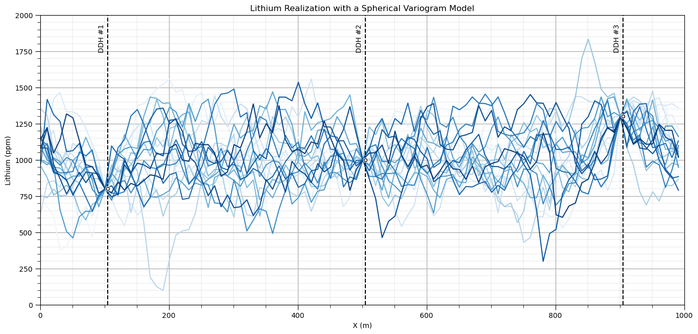
Spherical Variogram Model#
A very commonly observed variogram / spatial continuity form in many settings
Piecewise, beyond the range is equal to the sill
The equation:
where \(𝑐_1\) is the contribution, \(𝑎\) is the range and \(\bf{𝐡}\) is the lag distance
nreal = 20; vrange = 100                                      # number of realizations and variogram range

vario = GSLIB.make_variogram(nug=0.0,nst=1,it1=1,cc1=1.0,azi1=90.0,hmaj1=vrange,hmin1=5)

with io.capture_output() as captured:                         # simulation while muting output
    sim_spherical = geostats.sgsim(df,'X','Y','Lithium',wcol=-1,scol=-1,tmin=tmin,tmax=tmax,itrans=1,ismooth=0,
        dftrans=0,tcol=0,twtcol=0,zmin=0.0,zmax=2000.0,ltail=1,ltpar=0.0,utail=1,utpar=2000,nsim=nreal,
        nx=nx,xmn=xmn,xsiz=xsiz,ny=ny,ymn=ymn,ysiz=ysiz,seed=73074,ndmin=ndmin,ndmax=ndmax,nodmax=10,
        mults=0,nmult=2,noct=-1,ktype=0,colocorr=0.0,sec_map=0,vario=vario).reshape((20,100))

plt.subplot(111)                                              # plot variograms
for i in range(0, nreal):
    plt.plot(np.arange(1,(nx*xsiz),xsiz),sim_spherical[i],color=plt.cm.Blues(i/nreal),label='Real ' + str(i+1),zorder=1)

for idata in range(0,3):                                      # plot data
    plt.plot([df.loc[idata,'X'],df.loc[idata,'X']],[lithmin,lithmax],color='black',ls='--')
    plt.scatter(df.loc[idata,'X'],df.loc[idata,'Lithium'],s=20,color='white',edgecolor='black',zorder=10)
    plt.scatter(df.loc[idata,'X'],df.loc[idata,'Lithium'],s=40,color='white',edgecolor='white',zorder=9)
    plt.annotate(r'DDH #' + str(idata+1),(df.loc[idata,'X']-15,1750),rotation = 90);

plt.ylim([lithmin,lithmax]); plt.xlim([xmin,xmax]); add_grid()
plt.xlabel('X (m)'); plt.ylabel('Lithium (ppm)'); plt.title('Lithium Realization with a Spherical Variogram Model')

plt.subplots_adjust(left=0.0, bottom=0.0, right=2.0, top=1.2, wspace=0.2, hspace=0.2); plt.show()
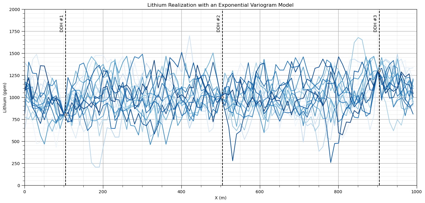
Exponential Variogram Model#
Also very commonly observed variogram / spatial continuity form
Less short-scale continuity than spherical, and reaches sill asymptotically, range is at 95% of the sill
The equation:
where \(𝑐_1\) is the contribution, \(𝑎\) is the range and \(\bf{h}\) is the lag distance.
nreal = 20; vrange = 100                                      # number of realizations and variogram range

vario = GSLIB.make_variogram(nug=0.0,nst=1,it1=2,cc1=1.0,azi1=90.0,hmaj1=vrange,hmin1=5)

with io.capture_output() as captured:                         # simulation while muting output
    sim_exponential = geostats.sgsim(df,'X','Y','Lithium',wcol=-1,scol=-1,tmin=tmin,tmax=tmax,itrans=1,ismooth=0,
        dftrans=0,tcol=0,twtcol=0,zmin=0.0,zmax=2000.0,ltail=1,ltpar=0.0,utail=1,utpar=2000,nsim=nreal,
        nx=nx,xmn=xmn,xsiz=xsiz,ny=ny,ymn=ymn,ysiz=ysiz,seed=73074,ndmin=ndmin,ndmax=ndmax,nodmax=10,
        mults=0,nmult=2,noct=-1,ktype=0,colocorr=0.0,sec_map=0,vario=vario).reshape((20,100))

plt.subplot(111)                                              # plot variograms
for i in range(0, nreal):
    plt.plot(np.arange(1,(nx*xsiz),xsiz),sim_exponential[i],color=plt.cm.Blues(i/nreal),label='Real ' + str(i+1),zorder=1)

for idata in range(0,3):                                      # plot data
    plt.plot([df.loc[idata,'X'],df.loc[idata,'X']],[lithmin,lithmax],color='black',ls='--')
    plt.scatter(df.loc[idata,'X'],df.loc[idata,'Lithium'],s=20,color='white',edgecolor='black',zorder=10)
    plt.scatter(df.loc[idata,'X'],df.loc[idata,'Lithium'],s=40,color='white',edgecolor='white',zorder=9)
    plt.annotate(r'DDH #' + str(idata+1),(df.loc[idata,'X']-15,1750),rotation = 90);

plt.ylim([lithmin,lithmax]); plt.xlim([xmin,xmax]); add_grid()
plt.xlabel('X (m)'); plt.ylabel('Lithium (ppm)'); plt.title('Lithium Realization with an Exponential Variogram Model')

plt.subplots_adjust(left=0.0, bottom=0.0, right=2.0, top=1.2, wspace=0.2, hspace=0.2); plt.show()
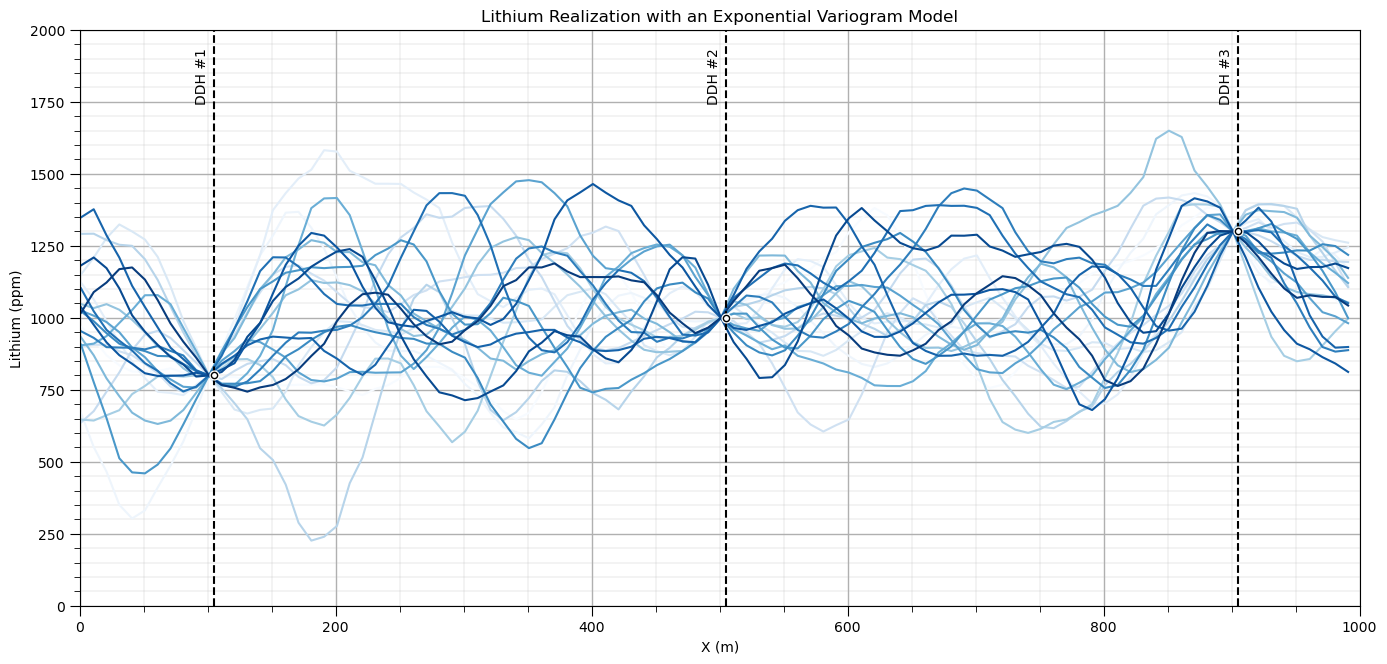
Gaussian Variogram Model#
Less commonly observed variogram / spatial continuity form, e.g., for thickness and elevation
Much more short-scale continuity than spherical, and reaches sill asymptotically, range is at 95% of the sill
The equation:
where \(𝑐_1\) is the contribution, \(𝑎\) is the range and \(\bf{h}\) is the lag distance.
nreal = 20; vrange = 100                                      # number of realizations and variogram range

vario = GSLIB.make_variogram(nug=0.001,nst=1,it1=3,cc1=0.999,azi1=90.0,hmaj1=100,hmin1=5)

with io.capture_output() as captured:                         # simulation while muting output
    sim_Gaussian = geostats.sgsim(df,'X','Y','Lithium',wcol=-1,scol=-1,tmin=tmin,tmax=tmax,itrans=1,ismooth=0,
        dftrans=0,tcol=0,twtcol=0,zmin=0.0,zmax=2000.0,ltail=1,ltpar=0.0,utail=1,utpar=2000,nsim=nreal,
        nx=nx,xmn=xmn,xsiz=xsiz,ny=ny,ymn=ymn,ysiz=ysiz,seed=73074,ndmin=ndmin,ndmax=ndmax,nodmax=10,
        mults=0,nmult=2,noct=-1,ktype=0,colocorr=0.0,sec_map=0,vario=vario).reshape((20,100))

plt.subplot(111)                                              # plot variograms
for i in range(0, nreal):
    plt.plot(np.arange(1,(nx*xsiz),xsiz),sim_Gaussian[i],color=plt.cm.Blues(i/nreal),label='Real ' + str(i+1),zorder=1)

for idata in range(0,3):                                      # plot data
    plt.plot([df.loc[idata,'X'],df.loc[idata,'X']],[lithmin,lithmax],color='black',ls='--')
    plt.scatter(df.loc[idata,'X'],df.loc[idata,'Lithium'],s=20,color='white',edgecolor='black',zorder=10)
    plt.scatter(df.loc[idata,'X'],df.loc[idata,'Lithium'],s=40,color='white',edgecolor='white',zorder=9)
    plt.annotate(r'DDH #' + str(idata+1),(df.loc[idata,'X']-15,1750),rotation = 90);

plt.ylim([lithmin,lithmax]); plt.xlim([xmin,xmax]); add_grid()
plt.xlabel('X (m)'); plt.ylabel('Lithium (ppm)'); plt.title('Lithium Realization with an Exponential Variogram Model')

plt.subplots_adjust(left=0.0, bottom=0.0, right=2.0, top=1.2, wspace=0.2, hspace=0.2); plt.show()
Vary the Variogram Model Type#
Let’s compare the variogram models by plotting them all together.
spherical
exponential
Gaussian
nreal = 20; vrange = 80                                       # number of realizations and variogram range
h = np.linspace(0,1000,100)

fig = plt.figure()
grid_spec = gridspec.GridSpec(ncols = 2,nrows=3,width_ratios=[1, 2])

ax0 = fig.add_subplot(grid_spec[0])
gamma_sph = 1.0*(1.5*h/vrange) - 0.5*np.power(h/vrange,3)
gamma_sph[h > vrange] = 1.0

plot = ax0.plot(h,gamma_sph,color='red',lw=4)
plt.plot([0,100],[1.0,1.0],color='black',ls='--'); plt.annotate('Sill',[5,1.02])
plt.plot([0,vrange*2/3],[0,1.0],color='black',ls='--'); plt.annotate(r'$\frac{2}{3}$ Range',[vrange*2/3,1.02])
plt.plot([vrange,vrange],[0.0,1.0],color='black',ls='--'); plt.annotate('Range',[vrange-6.5,0.4],rotation=90.0)
plt.xlim([0,140]); plt.ylim([0,1.2])
plt.xlabel(r'Lag Distance, $\bf{h}$'); plt.ylabel(r'Variogram, $\gamma$ ($\bf{h}$)')
plt.title('Spherical Variogram Model')

ax1 = fig.add_subplot(grid_spec[1])
vario = GSLIB.make_variogram(nug=0.0,nst=1,it1=1,cc1=1.0,azi1=90.0,hmaj1=vrange,hmin1=5)

with io.capture_output() as captured:                         # simulation while muting output
    sim_spherical = geostats.sgsim(df,'X','Y','Lithium',wcol=-1,scol=-1,tmin=tmin,tmax=tmax,itrans=1,ismooth=0,
        dftrans=0,tcol=0,twtcol=0,zmin=0.0,zmax=2000.0,ltail=1,ltpar=0.0,utail=1,utpar=2000,nsim=nreal,
        nx=nx,xmn=xmn,xsiz=xsiz,ny=ny,ymn=ymn,ysiz=ysiz,seed=73074,ndmin=ndmin,ndmax=ndmax,nodmax=10,
        mults=0,nmult=2,noct=-1,ktype=0,colocorr=0.0,sec_map=0,vario=vario).reshape((20,100))

for i in range(0, nreal):
    plt.plot(np.arange(1,(nx*xsiz),xsiz),sim_spherical[i],color=plt.cm.Blues(i/nreal),label='Real ' + str(i+1),zorder=1)

for idata in range(0,3):                                      # plot data
    plt.plot([df.loc[idata,'X'],df.loc[idata,'X']],[lithmin,lithmax],color='black',ls='--')
    plt.scatter(df.loc[idata,'X'],df.loc[idata,'Lithium'],s=20,color='white',edgecolor='black',zorder=10)
    plt.scatter(df.loc[idata,'X'],df.loc[idata,'Lithium'],s=40,color='white',edgecolor='white',zorder=9)
    plt.annotate(r'DDH #' + str(idata+1),(df.loc[idata,'X']-15,1750),rotation = 90);

plt.ylim([lithmin,lithmax]); plt.xlim([xmin,xmax]); add_grid()
plt.xlabel('X (m)'); plt.ylabel('Lithium (ppm)'); plt.title('Lithium Realization with a Spherical Variogram Model')

ax2 = fig.add_subplot(grid_spec[2])
gamma_exp = 1.0*(1.0-np.exp(-3*(h/vrange)))

plot = ax2.plot(h,gamma_exp,color='red',lw=4)
plt.plot([0,150],[1.0,1.0],color='black',ls='--'); plt.annotate('Sill',[5,1.02])
plt.plot([0,vrange],[0.95,0.95],color='grey',ls='-'); plt.annotate('95% Sill',[5,0.91])
plt.plot([vrange,vrange],[0.0,1.0],color='black',ls='--'); plt.annotate('Range',[vrange-6.5,0.4],rotation=90.0)
plt.plot([0,vrange*1/3],[0,1.0],color='black',ls='--'); plt.annotate(r'$\frac{1}{3}$ Range',[vrange*1/3,1.02])
plt.xlim([0,140]); plt.ylim([0,1.2])
plt.xlabel(r'Lag Distance, $\bf{h}$'); plt.ylabel(r'Variogram, $\gamma$ ($\bf{h}$)')
plt.title('Exponential Variogram Model')

ax3 = fig.add_subplot(grid_spec[3])
vario = GSLIB.make_variogram(nug=0.0,nst=1,it1=2,cc1=1.0,azi1=90.0,hmaj1=vrange,hmin1=5)

with io.capture_output() as captured:                         # simulation while muting output
    sim_exponential = geostats.sgsim(df,'X','Y','Lithium',wcol=-1,scol=-1,tmin=tmin,tmax=tmax,itrans=1,ismooth=0,
        dftrans=0,tcol=0,twtcol=0,zmin=0.0,zmax=2000.0,ltail=1,ltpar=0.0,utail=1,utpar=2000,nsim=nreal,
        nx=nx,xmn=xmn,xsiz=xsiz,ny=ny,ymn=ymn,ysiz=ysiz,seed=73074,ndmin=ndmin,ndmax=ndmax,nodmax=10,
        mults=0,nmult=2,noct=-1,ktype=0,colocorr=0.0,sec_map=0,vario=vario).reshape((20,100))

for i in range(0, nreal):
    plt.plot(np.arange(1,(nx*xsiz),xsiz),sim_exponential[i],color=plt.cm.Blues(i/nreal),label='Real ' + str(i+1),zorder=1)

for idata in range(0,3):                                      # plot data
    plt.plot([df.loc[idata,'X'],df.loc[idata,'X']],[lithmin,lithmax],color='black',ls='--')
    plt.scatter(df.loc[idata,'X'],df.loc[idata,'Lithium'],s=20,color='white',edgecolor='black',zorder=10)
    plt.scatter(df.loc[idata,'X'],df.loc[idata,'Lithium'],s=40,color='white',edgecolor='white',zorder=9)
    plt.annotate(r'DDH #' + str(idata+1),(df.loc[idata,'X']-15,1750),rotation = 90);

plt.ylim([lithmin,lithmax]); plt.xlim([xmin,xmax]); add_grid()
plt.xlabel('X (m)'); plt.ylabel('Lithium (ppm)'); plt.title('Lithium Realization with an Exponential Variogram Model')

ax4 = fig.add_subplot(grid_spec[4])
gamma_gaus = 1.0*(1.0-np.exp(-3*np.power(h/vrange,2)))

plot = ax4.plot(h,gamma_gaus,color='red',lw=4)
plt.plot([0,150],[1.0,1.0],color='black',ls='--'); plt.annotate('Sill',[5,1.02])
plt.plot([0,vrange],[0.95,0.95],color='grey',ls='-'); plt.annotate('95% Sill',[5,0.91])
plt.plot([vrange,vrange],[0.0,1.0],color='black',ls='--'); plt.annotate('Range',[vrange-6.5,0.4],rotation=90.0)
plt.xlim([0,140]); plt.ylim([0,1.2])
plt.xlabel(r'Lag Distance, $\bf{h}$'); plt.ylabel(r'Variogram, $\gamma$ ($\bf{h}$)')
plt.title('Gaussian Variogram Model')

ax5 = fig.add_subplot(grid_spec[5])
vario = GSLIB.make_variogram(nug=0.001,nst=1,it1=3,cc1=0.999,azi1=90.0,hmaj1=100,hmin1=5)

with io.capture_output() as captured:                         # simulation while muting output
    sim_Gaussian = geostats.sgsim(df,'X','Y','Lithium',wcol=-1,scol=-1,tmin=tmin,tmax=tmax,itrans=1,ismooth=0,
        dftrans=0,tcol=0,twtcol=0,zmin=0.0,zmax=2000.0,ltail=1,ltpar=0.0,utail=1,utpar=2000,nsim=nreal,
        nx=nx,xmn=xmn,xsiz=xsiz,ny=ny,ymn=ymn,ysiz=ysiz,seed=73074,ndmin=ndmin,ndmax=ndmax,nodmax=10,
        mults=0,nmult=2,noct=-1,ktype=0,colocorr=0.0,sec_map=0,vario=vario).reshape((20,100))

for i in range(0, nreal):
    plt.plot(np.arange(1,(nx*xsiz),xsiz),sim_Gaussian[i],color=plt.cm.Blues(i/nreal),label='Real ' + str(i+1),zorder=1)

for idata in range(0,3):                                      # plot data
    plt.plot([df.loc[idata,'X'],df.loc[idata,'X']],[lithmin,lithmax],color='black',ls='--')
    plt.scatter(df.loc[idata,'X'],df.loc[idata,'Lithium'],s=20,color='white',edgecolor='black',zorder=10)
    plt.scatter(df.loc[idata,'X'],df.loc[idata,'Lithium'],s=40,color='white',edgecolor='white',zorder=9)
    plt.annotate(r'DDH #' + str(idata+1),(df.loc[idata,'X']-15,1750),rotation = 90);

plt.ylim([lithmin,lithmax]); plt.xlim([xmin,xmax]); add_grid()
plt.xlabel('X (m)'); plt.ylabel('Lithium (ppm)'); plt.title('Lithium Realization with an Exponential Variogram Model')

plt.subplots_adjust(left=0.0, bottom=0.0, right=2.0, top=3.1, wspace=0.2, hspace=0.2); plt.show()
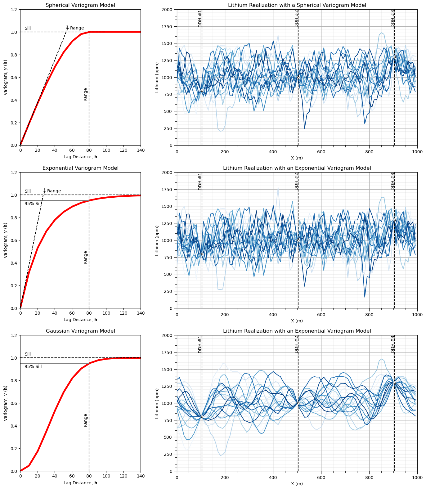
There is a clear difference in short scale continuity, with increasing short scale spatial continuity from exponential to spherical to Gaussian. But the long range spatial continuity does not change significantly.
Vary the Nugget Effect#
Now’s let’s use the same spherical variogram model with constant range and just vary the relative nugget effect:
0% relative nugget effect
50% relative nugget effect
90% relative nugget effect
nreal = 20; vrange = 120                                      # number of realizations and variogram range
nugget = [0.0,0.5,0.9]                                        # relative nugget effects

fig = plt.figure()
grid_spec = gridspec.GridSpec(ncols = 2,nrows=3,width_ratios=[1, 2])

for inug in range(0,len(nugget)):

    ax0 = fig.add_subplot(grid_spec[inug*2])
    gamma_sph = (1.0-nugget[inug])*((1.5*h/vrange) - 0.5*np.power(h/vrange,3))+nugget[inug]
    gamma_sph[h > vrange] = 1.0

    plot = ax0.plot(h,gamma_sph,color='red',lw=4)             # plot the variogram model
    plt.plot([0,100],[1.0,1.0],color='black',ls='--'); plt.annotate('Sill',[5,1.02])
    plt.plot([0,vrange*2/3],[nugget[inug],1.0],color='black',ls='--'); plt.annotate(r'$\frac{2}{3}$ Range',[vrange*2/3,1.02])
    plt.plot([vrange,vrange],[0.0,1.0],color='black',ls='--'); plt.annotate('Range',[vrange-6.5,0.4],rotation=90.0)
    plt.xlim([0,140]); plt.ylim([0,1.2])
    plt.xlabel(r'Lag Distance, $\bf{h}$'); plt.ylabel(r'Variogram, $\gamma$ ($\bf{h}$)')
    plt.title('Spherical Variogram Model')

    ax1 = fig.add_subplot(grid_spec[inug*2+1])
    vario = GSLIB.make_variogram(nug=nugget[inug],nst=1,it1=1,cc1=1.0-nugget[inug],azi1=90.0,hmaj1=vrange,hmin1=5)

    with io.capture_output() as captured:                     # calculate the simulated realizations
        sim_spherical = geostats.sgsim(df,'X','Y','Lithium',wcol=-1,scol=-1,tmin=tmin,tmax=tmax,itrans=1,ismooth=0,
            dftrans=0,tcol=0,twtcol=0,zmin=0.0,zmax=2000.0,ltail=1,ltpar=0.0,utail=1,utpar=2000,nsim=nreal,
            nx=nx,xmn=xmn,xsiz=xsiz,ny=ny,ymn=ymn,ysiz=ysiz,seed=73074,ndmin=ndmin,ndmax=ndmax,nodmax=10,
            mults=0,nmult=2,noct=-1,ktype=0,colocorr=0.0,sec_map=0,vario=vario).reshape((20,100))

    for i in range(0, nreal):
        plt.plot(np.arange(1,(nx*xsiz),xsiz),sim_spherical[i],color=plt.cm.Blues(i/nreal),label='Real ' + str(i+1),zorder=1)

    for idata in range(0,3):                                  # plot the simulated realizations
        plt.plot([df.loc[idata,'X'],df.loc[idata,'X']],[lithmin,lithmax],color='black',ls='--')
        plt.scatter(df.loc[idata,'X'],df.loc[idata,'Lithium'],s=20,color='white',edgecolor='black',zorder=10)
        plt.scatter(df.loc[idata,'X'],df.loc[idata,'Lithium'],s=40,color='white',edgecolor='white',zorder=9)
        plt.annotate(r'DDH #' + str(idata+1),(df.loc[idata,'X']-15,1750),rotation = 90);

    plt.ylim([lithmin,lithmax]); plt.xlim([xmin,xmax]); add_grid()
    plt.xlabel('X (m)'); plt.ylabel('Lithium (ppm)');
    plt.title('Lithium Realization with a Spherical Variogram Model, ' + str(nugget[inug]) + ' Relative Nugget Effect')

plt.subplots_adjust(left=0.0, bottom=0.0, right=2.0, top=3.1, wspace=0.2, hspace=0.2); plt.show()
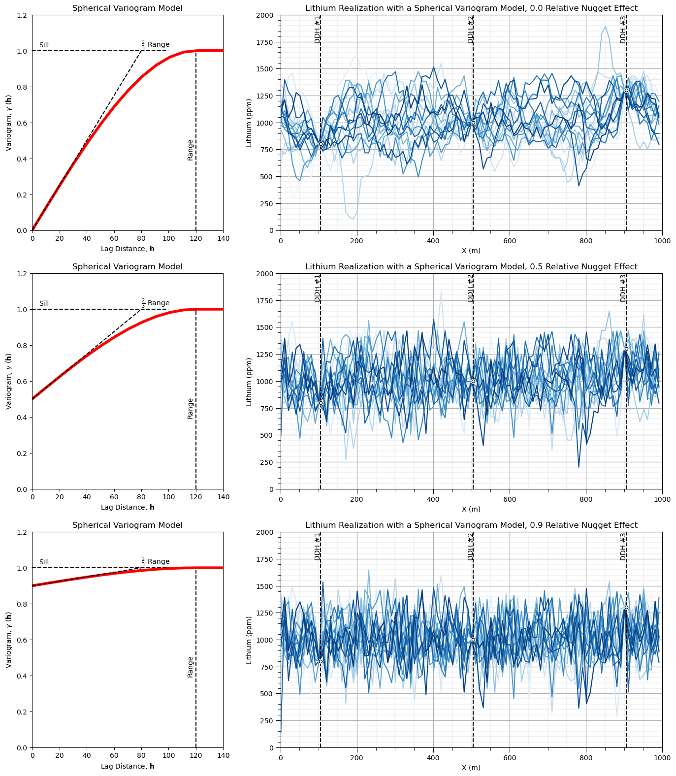
There is a clear difference in short scale continuity, with decreasing short scale spatial continuity with increase in relative nugget effect.
About the Author#

Michael Pyrcz is a professor in the Cockrell School of Engineering, and the Jackson School of Geosciences, at The University of Texas at Austin, where he researches and teaches subsurface, spatial data analytics, geostatistics, and machine learning. Michael is also,
the principal investigator of the Energy Analytics freshmen research initiative and a core faculty in the Machine Learn Laboratory in the College of Natural Sciences, The University of Texas at Austin
an associate editor for Computers and Geosciences, and a board member for Mathematical Geosciences, the International Association for Mathematical Geosciences.
Michael has written over 70 peer-reviewed publications, a Python package for spatial data analytics, co-authored a textbook on spatial data analytics, Geostatistical Reservoir Modeling and author of two recently released e-books, Applied Geostatistics in Python: a Hands-on Guide with GeostatsPy and Applied Machine Learning in Python: a Hands-on Guide with Code.
All of Michael’s university lectures are available on his YouTube Channel with links to 100s of Python interactive dashboards and well-documented workflows in over 40 repositories on his GitHub account, to support any interested students and working professionals with evergreen content. To find out more about Michael’s work and shared educational resources visit his Website.
Want to Work Together?#
I hope this content is helpful to those that want to learn more about subsurface modeling, data analytics and machine learning. Students and working professionals are welcome to participate.
Want to invite me to visit your company for training, mentoring, project review, workflow design and / or consulting? I’d be happy to drop by and work with you!
Interested in partnering, supporting my graduate student research or my Subsurface Data Analytics and Machine Learning consortium (co-PI is Professor John Foster)? My research combines data analytics, stochastic modeling and machine learning theory with practice to develop novel methods and workflows to add value. We are solving challenging subsurface problems!
I can be reached at mpyrcz@austin.utexas.edu.
I’m always happy to discuss,
Michael
Michael Pyrcz, Ph.D., P.Eng. Professor, Cockrell School of Engineering and The Jackson School of Geosciences, The University of Texas at Austin
More Resources Available at: Twitter | GitHub | Website | GoogleScholar | Geostatistics Book | YouTube | Applied Geostats in Python e-book | Applied Machine Learning in Python e-book | LinkedIn
Comments#
This was a basic demonstration of variogram calculation with GeostatsPy. Much more can be done, I have other demonstrations for modeling workflows with GeostatsPy in the GitHub repository GeostatsPy_Demos.
I hope this is helpful,
Michael