Heterogeneity Metrics

Heterogeneity Metrics#

Michael J. Pyrcz, Professor, The University of Texas at Austin

Chapter of e-book “Applied Geostatistics in Python: a Hands-on Guide with GeostatsPy”.

Cite this e-Book as:

Pyrcz, M.J., 2024, Applied Geostatistics in Python: a Hands-on Guide with GeostatsPy [e-book]. Zenodo. doi:10.5281/zenodo.15169133

The workflows in this book and more are available here:

Cite the GeostatsPyDemos GitHub Repository as:

Pyrcz, M.J., 2024, GeostatsPyDemos: GeostatsPy Python Package for Spatial Data Analytics and Geostatistics Demonstration Workflows Repository (0.0.1) [Software]. Zenodo. doi:10.5281/zenodo.12667036. GitHub Repository: GeostatsGuy/GeostatsPyDemos

By Michael J. Pyrcz
© Copyright 2024.

This chapter is a tutorial for / demonstration of Heterogeneity Metrics.

YouTube Lecture: check out my lecture on:

Heterogeneity Metrics

These lectures are all part of my Data Analytics and Geostatistics Course on YouTube with linked well-documented Python workflows and interactive dashboards. My goal is to share accessible, actionable, and repeatable educational content. If you want to know about my motivation, check out Michael’s Story.

Motivation#

There is a vast difference in heterogeneity of reservoirs,

heterogeneity is the change in features over location or time
conversely, homogeneity is the consistency of variables over location or time

Heterogeneity impacts the recovery of hydrocarbons from the reservoir, minerals from ore bodies and water from aquifers,

we need metrics to quantify the heterogeneity in our subsurface data and subsurface models

Applications with Measures of Heterogeneity#

Measures of heterogeneity are often applied proxy, approximate measures to indicate reservoir production / performance.
These measures may be applied to compare and rank reservoirs or reservoir model realizations for a single reservoir.

Best Practice#

None of these metrics are perfect.
The best result possible from rigorous flow forecasting applied to good, full 3D reservoir models, use the physics when possible!
Integrate all relevant information, at sufficient scale to resolve important features

Caution#

Use of simple heterogeneity measures for ranking reservoir and reservoir models can be dangerous.
Inaccuracy can result in incorrect rank estimates; therefore, incorrect business decisions.

Other Measures#

We just consider simple, static measures here
I also have a Python demonstration for Lorenz coefficient
Got your own measure? You may develop a new metric. Novel methods for quantifying heterogeneity within reservoirs is a currently active area of research.

Load the Required Libraries#

The following code loads the required libraries.

ignore_warnings = True                                        # ignore warnings?
import numpy as np                                            # arrays
import pandas as pd                                           # dataframes
import scipy.stats as stats                                   # statistical functions
from scipy.integrate import quad                              # for numerical integration
import math                                                   # square root to calculate standard deviation from variance
import matplotlib.pyplot as plt                               # plotting
from matplotlib.ticker import (MultipleLocator, AutoMinorLocator) # control of axes ticks
import matplotlib.ticker as mtick                             # control tick label formatting
plt.rc('axes', axisbelow=True)                                # plot all grids below the plot elements
if ignore_warnings == True:                                   
    import warnings
    warnings.filterwarnings('ignore')
cmap = plt.cm.inferno                                         # color map
seed = 42                                                     # random number seed

If you get a package import error, you may have to first install some of these packages. This can usually be accomplished by opening up a command window on Windows and then typing ‘python -m pip install [package-name]’. More assistance is available with the respective package docs.

Define Functions#

This is a convenience function to add major and minor gridlines to improve plot interpretability.

def add_grid():
    plt.gca().grid(True, which='major',linewidth = 1.0); plt.gca().grid(True, which='minor',linewidth = 0.2) # add y grids
    plt.gca().tick_params(which='major',length=7); plt.gca().tick_params(which='minor', length=4)
    plt.gca().xaxis.set_minor_locator(AutoMinorLocator()); plt.gca().yaxis.set_minor_locator(AutoMinorLocator()) # turn on minor ticks

Set the working directory#

I always like to do this so I don’t lose files and to simplify subsequent read and writes (avoid including the full address each time).

#os.chdir("c:/PGE383/Examples")             # set the working directory

Loading Tabular Data#

Here’s the command to load our comma delimited data file in to a Pandas’ DataFrame object.

we will use this spatial dataset for our heterogeneity metrics up to Lorenz coefficient, for this Lorenz coefficient load a single well with porosity and permeability features

df = pd.read_csv('https://raw.githubusercontent.com/GeostatsGuy/GeoDataSets/master/PorPermSample1.csv')
df.head()

	Depth	Porosity	Perm
0	0.25	12.993634	265.528738
1	0.50	13.588011	116.891220
2	0.75	8.962625	136.920016
3	1.00	17.634879	216.668629
4	1.25	9.424404	131.594114

Feature Engineering#

We will need to make a new feature, approximate rock quality index, the ratio of permeability divided by porosity.

rock quality index (RQI) approximation - the formula for calculating RQI includes permeability divided by porosity and is commonly used to identify rock groups, like facies. While we only use the permeability divided by porosity ratio, the complete equation for RQI is,

\[ RQI = 0.0314 \times \sqrt{\frac{k}{\phi}} \]

df['PermPor'] = df['Perm'].values/df['Porosity'].values       # new feature as permability divided by porosity
df.head()

	Depth	Porosity	Perm	PermPor
0	0.25	12.993634	265.528738	20.435295
1	0.50	13.588011	116.891220	8.602526
2	0.75	8.962625	136.920016	15.276776
3	1.00	17.634879	216.668629	12.286369
4	1.25	9.424404	131.594114	13.963124

Variance of Permeability#

It is common to use the sample or population variance of permeability as a measure of heterogeneity. I demonstrate the sample variance.

\begin{equation} \sigma_{X_k}^2 = \frac{1}{n} \sum_{i=1}^{n-1} (x_{k,i} - \overline{x_k})^2 \end{equation}

var_perm = np.var(df['Perm'].values,ddof=1)                   # sample variance of permeability 
print('Sample Variance of Permeability: ' + str(np.round(var_perm,2)) + ' mD^2')

Sample Variance of Permeability: 6544.83 mD^2

Coefficient of Variation of Permeability#

Another common heternogeneity metric is the coefficient of variation, the standard deviation standardized by the mean.

\begin{equation} C_{v_k} = \frac{\sigma_k}{\overline{k} } \end{equation}

Note, by specifying the ddof arguement of 1, we are using the sample standard deviation in the calculation.

coefvar_perm = stats.variation(df['Perm'].values,ddof=1)      # coefficient of variation of permeability
print('Coefficeint of Variation of Permeability: ' + str(np.round(coefvar_perm,3)) + ' unitless')

Coefficeint of Variation of Permeability: 0.502 unitless

Coefficient of Variation of Permeability / Porosity#

Also it is common to calculate the coefficient of variation of the ratio of permeability divided by porosity.

\begin{equation} C_{v_\frac{k}{\phi}} = \frac{\sigma_{\frac{k}{\phi}}}{\overline{\frac{k}{\phi}} } \end{equation}

coefvar_permpor = stats.variation(df['PermPor'].values,ddof=1) # coefficient of variation of permeability divided by porosity
print('Coefficient of Variation of Permeability / Porosity: ' + str(np.round(coefvar_permpor,3)) + ' unitless')

Coefficient of Variation of Permeability / Porosity: 0.369 unitless

Dykstra Parsons#

Now let’s calculate the Dykstra-Parsons coefficient.

\begin{equation} DP = \frac{P50_k - P16_k}{P50_k} \end{equation}

P16_perm = np.percentile(df['Perm'].values,16)                # the permeability 16th percentile
P50_perm = np.percentile(df['Perm'].values,50)                # the permeability 50th percentile (median)

print('Permeability P16: ' + str(np.round(P16_perm,3)))
print('Permeability P50: ' + str(np.round(P50_perm,3)))

dp = (P50_perm - P16_perm)/P50_perm                           # Dykstra Parsons
print('\nDykstra-Parsons Coefficient: ' + str(np.round(dp,3)) + ' unitless')

Permeability P16: 84.797
Permeability P50: 144.33

Dykstra-Parsons Coefficient: 0.412 unitless

Dykstra-Parsons Improved by Fitting a Lognormal Distribution to Permeability#

We may be able to improve our Dykstra-Parsons coefficient calculation by fitting a lognormal distibution to permeability and then using the parametric lognormal distribution to get a more accurate estimate of the P50 and P16 or permeability.

calculate the lognormal parameters, \mu (mu) and \sigma (sigma)
use the parametric lognormal CDF inverse to get the P50 and P16

mean_perm = np.average(df['Perm'].values)                     # average of permeability

mu = np.log((mean_perm**2)/math.sqrt(var_perm + mean_perm**2)) # given the average and variance, calculate the associated lognormal mu and sigma
sigma = math.sqrt(np.log(var_perm/(mean_perm**2)+1))

print('Lognormal distribution parameters are, mu: ' + str(np.round(mu,2)) + ', and sigma: ' + str(np.round(sigma,2)))

Lognormal distribution parameters are, mu: 4.97, and sigma: 0.47

Now we can calculate the P50 and P16 of permeability from the fit lognormal distribution.

Note, we could have been more rigorous with our distribution fit with a ordinary least squares or maximum likelihood approach.

P16_perm_lognorm = stats.lognorm.ppf(0.16,s = sigma, scale = math.exp(mu)) # calculate permeability P16 and P50 from our estimated lognormal distribution
P50_perm_lognorm = stats.lognorm.ppf(0.50,s = sigma, scale = math.exp(mu))

print('Permeability P16 from Lognormal Parametric Distribution: ' + str(np.round(P16_perm_lognorm,3)))
print('Permeability P50 from Lognormal Parametric Distribution: ' + str(np.round(P50_perm_lognorm,3)))

Permeability P16 from Lognormal Parametric Distribution: 89.754
Permeability P50 from Lognormal Parametric Distribution: 143.869

dp_lognorm = (P50_perm_lognorm - P16_perm_lognorm)/P50_perm_lognorm # Dykstra-Parsons coefficient
print('\nDykstra-Parsons Coefficient: ' + str(np.round(dp_lognorm,3)) + ' unitless')

Dykstra-Parsons Coefficient: 0.376 unitless

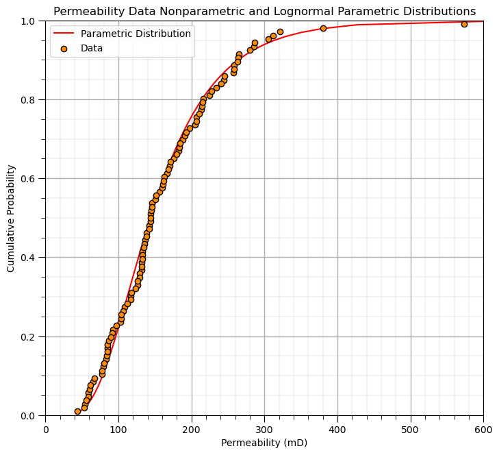
Visualize the Lognormal Permeability Parametric Distribution#

Let’s check our lognormal parametric distribution fit.

we visualize the lognormal parametric CDF and the permeability data nonparametric distribution together to check the fit

cumul_prob = np.linspace(0.01,0.999,100)                      # get points on our estimated lognormal distribution
lognormal = stats.lognorm.ppf(cumul_prob,s = sigma, scale = math.exp(mu))

plt.plot(lognormal,cumul_prob,color='red',label='Parametric Distribution',zorder=1)
plt.xlabel('Permeability (mD)'); plt.ylabel('Cumulative Probability'); plt.title('Permeability Data Nonparametric and Lognormal Parametric Distributions')
plt.ylim([0,1]); plt.xlim([0,600]); plt.grid()
plt.scatter(df['Perm'].values,df["Perm"].rank()/(len(df)+1),color='darkorange',edgecolor='black',zorder=10,label='Data')
plt.legend(loc='upper left'); add_grid()

plt.subplots_adjust(left=0.0, bottom=0.0, right=1.0, top=1.2, wspace=0.3, hspace=0.4); plt.show()

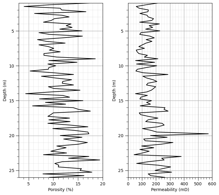
_images/4c6110c7cc6f4d7440521b83760417e910a647881ef1b042e014ac2d9485cc8f.png

Load a Single Well#

For the Lorenz coefficient we work with the statistics of stacked stratigraphic units in a single well.

we could sumarize the Lorenz coefficient over many wells but this would require a more complicated geological modeling workflow.

df_well = pd.read_csv('https://raw.githubusercontent.com/GeostatsGuy/GeoDataSets/master/WellPorPermSample_3.csv') 
df_well = df_well.rename(columns={"Depth (m)":"Depth", "Por (%)":"Por", "Perm (mD)":"Perm"})
nwell = len(df_well)
print('Number of samples in the well = ' + str(nwell))

plt.subplot(121)
plt.plot(df_well['Por'],df_well['Depth'],color='black'); add_grid(); plt.xlabel('Porosity (%)'); plt.ylabel('Depth (m)')
plt.ylim([26,1]); plt.xlim([3,20])

plt.subplot(122)
plt.plot(df_well['Perm'],df_well['Depth'],color='black'); add_grid(); plt.xlabel('Permeability (mD)'); plt.ylabel('Depth (m)')
plt.ylim([26,1]); plt.xlim([0,600])

plt.subplots_adjust(left=0.0, bottom=0.0, right=1.0, top=1.2, wspace=0.3, hspace=0.4); plt.show()

Number of samples in the well = 105

_images/e91dd3871644e56fc799e5057d43955e0515e23fdab2cbd5e659a1c80ffd7e5f.png

Lorenz Coefficient Method#

1. Feature Engineering#

To prepare for the calculation of Lorenz Coefficient we need,

thickness - the thickness of eacch unit, in this case we observed equal thickness units at 0.25 m
rock quality index (RQI) approximation - once again we approximate RQI with only the ratio of permeability divided by porosity. For our application here we only need to sort the rock in descending rock quality index, so the square root and constant term would not change this order.

\(\quad\) since the square root and constant do not impact the order after sorting (below) we leave them out for brevity.

df_well['Thick'] = np.full(len(df_well),0.25)
df_well['PermPor'] = df_well['Perm']/df_well['Por']
df_well.head()

	Depth	Por	Perm	Thick	PermPor
0	0.25	13.0	265.5	0.25	20.423077
1	0.50	13.6	116.9	0.25	8.595588
2	0.75	9.0	136.9	0.25	15.211111
3	1.00	17.6	216.7	0.25	12.312500
4	1.25	9.4	131.6	0.25	14.000000

2. Sort the Data in Descending#

df_well = df_well.sort_values('PermPor',ascending = False)                   # sort in descending order
df_well.head()

	Depth	Por	Perm	Thick	PermPor
78	19.75	17.2	573.5	0.25	33.343023
103	26.00	9.2	263.5	0.25	28.641304
97	24.50	11.0	305.1	0.25	27.736364
72	18.25	8.9	244.1	0.25	27.426966
91	23.00	17.2	380.1	0.25	22.098837

3. Calculate Storage and Flow Capacities#

We calculate these as, storage capacity (SC),

\[ \text{SC} = \phi \times \text{Th} \]

and flow capacity (FC),

\[ \text{FC} = k \times \text{Th} \]

df_well['Storage'] = df_well['Por'] * df_well['Thick']
df_well['Flow'] = df_well['Perm'] * df_well['Thick']
df_well.head()

	Depth	Por	Perm	Thick	PermPor	Storage	Flow
78	19.75	17.2	573.5	0.25	33.343023	4.300	143.375
103	26.00	9.2	263.5	0.25	28.641304	2.300	65.875
97	24.50	11.0	305.1	0.25	27.736364	2.750	76.275
72	18.25	8.9	244.1	0.25	27.426966	2.225	61.025
91	23.00	17.2	380.1	0.25	22.098837	4.300	95.025

4. Calculate the Cumulative Storage and Flow Capacities#

We apply the cummulative sum down each column, storage capacity and flow capacity.

df_well['Storage_Cumul'] = df_well['Storage'].cumsum()
df_well['Flow_Cumul'] = df_well['Flow'].cumsum()
df_well.head()

	Depth	Por	Perm	Thick	PermPor	Storage	Flow	Storage_Cumul	Flow_Cumul
78	19.75	17.2	573.5	0.25	33.343023	4.300	143.375	4.300	143.375
103	26.00	9.2	263.5	0.25	28.641304	2.300	65.875	6.600	209.250
97	24.50	11.0	305.1	0.25	27.736364	2.750	76.275	9.350	285.525
72	18.25	8.9	244.1	0.25	27.426966	2.225	61.025	11.575	346.550
91	23.00	17.2	380.1	0.25	22.098837	4.300	95.025	15.875	441.575

5. Calculate the Cumulative Fraction of Storage and Flow Capacities#

We divide the storage and flow capacities by the largest value, i.e., the value in the last row, so that our statistics represent the fraction of the total cumulative.

df_well['Storage_Cumul_Frac'] = df_well['Storage_Cumul'] / df_well['Storage_Cumul'].max()
df_well['Flow_Cumul_Frac'] = df_well['Flow_Cumul'] / df_well['Flow_Cumul'].max()
df_well.head()

	Depth	Por	Perm	Thick	PermPor	Storage	Flow	Storage_Cumul	Flow_Cumul	Storage_Cumul_Frac	Flow_Cumul_Frac
78	19.75	17.2	573.5	0.25	33.343023	4.300	143.375	4.300	143.375	0.014024	0.033922
103	26.00	9.2	263.5	0.25	28.641304	2.300	65.875	6.600	209.250	0.021525	0.049508
97	24.50	11.0	305.1	0.25	27.736364	2.750	76.275	9.350	285.525	0.030493	0.067555
72	18.25	8.9	244.1	0.25	27.426966	2.225	61.025	11.575	346.550	0.037750	0.081994
91	23.00	17.2	380.1	0.25	22.098837	4.300	95.025	15.875	441.575	0.051773	0.104476

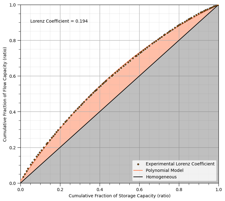
6. Calculate the Lorenz Coefficient#

This code may look a bit complicated, but the steps are simply,

Lorez Curve Model - fit a ploynomial (3rd order is sufficient) to the experimental Lorenz curve points
Lorenz Area - integrate between the fit polynomial curve and the homogeneous \(Y = X\) line
Lorenz Coefficient - divide by 0.5 to get the ratio of the Lorenz area divided by the total area above the homogeneous line

weights = np.ones(nwell)                                     
weights[0] = 1000; weights[-1] = 1000                 # to ensure the fit converges to (0,0) and (1,1)
    
coeffs = np.polyfit(df_well['Storage_Cumul_Frac'],df_well['Flow_Cumul_Frac'], deg=3, w=weights)
poly_fit = np.poly1d(coeffs)                          # create a polynomial function from the coefficients

def diff(x):
    return poly_fit(x) - x

lorenz_area, _ = quad(diff, a=0.0, b=1.0)

LC = np.round(lorenz_area/0.5,3)

plt.scatter(df_well['Storage_Cumul_Frac'],df_well['Flow_Cumul_Frac'],s=10,color='darkorange',edgecolor='black',label='Experimental Lorenz Coefficient',zorder=10)
plt.scatter(df_well['Storage_Cumul_Frac'],df_well['Flow_Cumul_Frac'],s=20,color='white',zorder=1)

plt.plot(np.linspace(0,1,100), poly_fit(np.linspace(0,1,100)),color='coral',zorder=5,label = 'Polynomial Model')

plt.annotate('Lorenz Coefficient = ' + str(LC),[0.05,0.9])

plt.fill_between(np.linspace(0,1,100), np.linspace(0,1,100),np.zeros(100), alpha = 0.5,facecolor='gray') 

plt.fill_between(np.linspace(0,1,100), poly_fit(np.linspace(0,1,100)),
                 np.linspace(0,1,100), alpha = 0.5,facecolor='coral',zorder=0) 

plt.xlim([0,1]); plt.ylim([0,1]); plt.xlabel('Cumulative Fraction of Storage Capacity (ratio)'); plt.ylabel('Cumulative Fraction of Flow Capacity (ratio)')
add_grid(); plt.plot([0,1],[0,1],color='black',label='Homogeneous'); plt.legend(loc='lower right')

plt.subplots_adjust(left=0.0, bottom=0.0, right=1.0, top=1.2, wspace=0.3, hspace=0.4); plt.show()

_images/685cd2d623b22a32b89522bf57bc1c58462a99aec31aae2583f7ecbe25eb6281.png

Comments#

This is a simple distribution of heterogeneity metrics. Much more could be done and discussed, I have many more resources. Check out my shared resource inventory and the YouTube lecture links at the start of this chapter with resource links in the videos’ descriptions.

I hope this is helpful,

Michael

About the Author#

Michael Pyrcz is a professor in the Cockrell School of Engineering, and the Jackson School of Geosciences, at The University of Texas at Austin, where he researches and teaches subsurface, spatial data analytics, geostatistics, and machine learning. Michael is also,

the principal investigator of the Energy Analytics freshmen research initiative and a core faculty in the Machine Learn Laboratory in the College of Natural Sciences, The University of Texas at Austin
an associate editor for Computers and Geosciences, and a board member for Mathematical Geosciences, the International Association for Mathematical Geosciences.

Michael has written over 70 peer-reviewed publications, a Python package for spatial data analytics, co-authored a textbook on spatial data analytics, Geostatistical Reservoir Modeling and author of two recently released e-books, Applied Geostatistics in Python: a Hands-on Guide with GeostatsPy and Applied Machine Learning in Python: a Hands-on Guide with Code.

All of Michael’s university lectures are available on his YouTube Channel with links to 100s of Python interactive dashboards and well-documented workflows in over 40 repositories on his GitHub account, to support any interested students and working professionals with evergreen content. To find out more about Michael’s work and shared educational resources visit his Website.

Want to Work Together?#

I hope this content is helpful to those that want to learn more about subsurface modeling, data analytics and machine learning. Students and working professionals are welcome to participate.

Want to invite me to visit your company for training, mentoring, project review, workflow design and / or consulting? I’d be happy to drop by and work with you!
Interested in partnering, supporting my graduate student research or my Subsurface Data Analytics and Machine Learning consortium (co-PIs including Profs. Foster, Torres-Verdin and van Oort)? My research combines data analytics, stochastic modeling and machine learning theory with practice to develop novel methods and workflows to add value. We are solving challenging subsurface problems!
I can be reached at mpyrcz@austin.utexas.edu.

I’m always happy to discuss,