
Probability Concepts#
Michael J. Pyrcz, Professor, The University of Texas at Austin
Twitter | GitHub | Website | GoogleScholar | Book | YouTube | Applied Geostats in Python e-book | LinkedIn
Chapter of e-book “Applied Geostatistics in Python: a Hands-on Guide with GeostatsPy”.
Cite this e-Book as:
Pyrcz, M.J., 2024, Applied Geostatistics in Python: a Hands-on Guide with GeostatsPy [e-book]. Zenodo. doi:10.5281/zenodo.15169133
The workflows in this book and more are available here:
Cite the GeostatsPyDemos GitHub Repository as:
Pyrcz, M.J., 2024, GeostatsPyDemos: GeostatsPy Python Package for Spatial Data Analytics and Geostatistics Demonstration Workflows Repository (0.0.1) [Software]. Zenodo. doi:10.5281/zenodo.12667036. GitHub Repository: GeostatsGuy/GeostatsPyDemos
By Michael J. Pyrcz
© Copyright 2024.
This chapter is a summary of Probability Concepts including essential concepts:
Motivation and Application to Model Uncertainty
Approaches to Calculate Probability
Probability Operators
Marginal, Conditional and Joint Probability
Independence Checks
Bayesian Updating
YouTube Lecture: check out my lectures on:
For convenience here’s a summary of the salient points.
Motivation for Probability#
Why cover probability at the beginning of a course on geostatistics?
Recall pillars of geostatistics from Geostatistical Concepts as a branch of applied statistics:
integrate geological context
account for spatial continuity
integrate scale (volume support) of data and models
focus on modeling uncertainty
Let us focus on this last point, uncertainty modeling. Probability is the fundamental approach to,
characterize uncertainty
model uncertainty
communicate uncertainty
In fact, the use of probability is entrenched in our shared language of uncertainty. Consider this fact,
the risk of dying while flying is 1 in 13.7 million per boarding world-wide; therefore, 0.000000073 probability
and we all use this probability (or just knowing this is an exceedingly small number) to frequently make the decision, that it is safe to fly,
at 700 - 900 kilometers per hour
at 30,000 - 42,000 feet in elevation (excuse the units mixing, in North America we think of elevation and our own height in feet)
inside a fuselage with an outer skin thickness of 1 millimeter aluminum
I hope I don’t sound jaded, as an engineer I’m respecting this engineering design and the resulting safety record. Let us brighten things up with this example,
given the local meteorologist’s estimate that there is a 95% chance of a sunny day tomorrow
you decide to drive your jeep (without a roof nor doors) to campus when leave for work in the early, dark hours of the morning. Full disclosure, I do have a change of clothes in my office just in case I make the wrong decision!
lecturing in wet clothes is awful, it happened before!
Probability
Probability is the language of uncertainty modeling and geostatistics is all about modeling uncertainty.
Now we get started by defining probability and then we will be ready to talk about ways to calculate it.
What is Probability?#
To understand what is probability consider Kolmogorov’s 3 axioms for probabilities, i.e., the rules that any measure of probability must honor,

non-negativity - probability of an event is a non-negative number
imagine negative probability!
normalization - probability of the entire sample space is one (unity), also known as probability closure
something happens!
additivity - addition of probability of mutually exclusive events for unions
e.g., probability of \(A_1\) and \(A_2\) mutual exclusive events is, \(Prob(A_1 + A_2) = Prob(A_1) + Prob(A_2)\)
note our concise notation, \(P(\cdot)\), for probabibility of event in the bracket occurring.
This is a good place to start for valid probabilities, we will refine this later. Now we can ask,
How to Calculate Probability?#
There are 3 probability perspectives that can be applied to calculate probabilities,
Probability by long-term frequencies (Frequentist Probability),
probability as ratio of outcomes from an experiment
requires repeated observations from a controlled experiment
for example, you flip a coin 100 times and count the number of outcomes with heads \(n(\text{heads})\) and then calculate this ratio,
this is the frequentist approach to calculate probabilities. The experiment is the set of coin tosses.
one issue with frequentist probabilities is, can we now use this probability of heads outside the experiment? For example,
on another day?
a different person tossing the coin?
a different coin?
Probability by physical tendencies or propensities (Engineering Probability),
probability calculated from knowledge about the system
we could know the probability of coin toss outcomes without the experiment
this is the engineering approach to probability, model the system and use this model, i.e., the physics of the system to calculate probability of outcomes
did you know that there is a \(\frac{1}{6,000}\) probability of a coin landing and staying upright on its edge? This could be lower depending of manner of tossing, coin thickness and characteristics of the surface.
Probability by Degrees of belief (Bayesian Probability),
first we specify the scientific concept of “belief” as your opinion based on all your knowledge and experience.
our model integrates our certainty about a result and data
this is very flexible, we can assign probability to any event, and includes a framework for updating with new information
if this is your approach, then you are using the Bayesian approach for probability. If not, before you dismiss this approach let me make a couple arguments,
you may be bothered by this idea of belief, as it may seem subjective compared to the probabilities objectively measured from a frequentist’s experiment but,
to use the frequentist probability you have to make the subjective decision to apply it outside the experiment, i.e., we need to go beyond a single coin!
the Bayesian probability approach includes objective probabilities from experiments, but it also allows for integration of our expert knowledge
A Warning about Calculating Probability#
Statistics can be misused or even abused, leading to flawed conclusions and poor decision-making. When probabilities are calculated improperly or misinterpreted, it can result in significant consequences. Here are a few examples of what can go wrong:
Insufficient sampling - there are various rules of thumb about what constitutes a small sample size, i.e., too small for inference about the population parameters and too small to train a reliable prediction model. Some say 7, some say 30, indubitably there is a minimum sample size.
in general, our models will communicate increasing uncertainty as the number of data decreases, but at some point these models break!
consider bootstrap, yes as the number of samples decrease the uncertainty in the statistic reported by bootstrap increases, but this uncertainty distribution is centered on the sample statistic! In other words, we need enough samples to have a reasonable estimate of the uncertainty model’s expectation in the first place.
of course, there is minimum number of samples to complete a mathematical operation, for example principal components analysis can only calculate \(n-1\) principal components (where \(n\) is the number of samples) and we cannot fit a linear regression model to \(n=1\) samples. Best practice is to stay very far away (have many more samples) from any of these algorithm limitations.
Biased sampling - in general our probability calculations will not automatically debias the sample data. Any bias in the samples will pass bias through to the probabilities representing our uncertainty model.
for example, a biased sample mean will bias simple kriging estimates away from data. Geostatistical simulation reproduces the entire input feature distribution, so any bias in any part of the distribution will be passed to the spatial models.
also, there is bad data. When we use Bayesian methods and rely on expert experience, that is not a license to say anything and defend it as belief. On the contrary, we must rigorously document and defend all our choices
Unskilled practice and a lack of rigor - there are mistakes that can be made with probabilities and some of them are shockingly common.
our first line of defense is to understand what our methods are doing under the hood! This will help us recognize logical inconsistencies as we build our workflows.
our second line of defense is to check every step in our workflows. Like an accountant we must close the loops with all our probability calculations, a process that accountants call reconciliation. Like a software engineer we must unit test every operation to ensure we don’t introduce errors as we update our probability workflows.
for example, if we perform primary feature cosimulation with the same random number seed as the secondary feature simulation we will introduce artificial correlation between the simulated primary and secondary features that will dramatically change the conditional and joint probabilities.
in another example, if we use information from the likelihood probabilities to inform the prior probabilities, we will significantly under-estimate the uncertainty. This error is a form of information leakage, descriptively we state it as “double dipping” from the information.
Please remember these warnings as you proceed below and onward as you build your own data science workflows.
Venn Diagrams#
Venn Diagrams are a tool to communicate probability.
representing the possible events or outcomes (\(A, B,\ldots\)) of an experiment within the collection of all possible events or outcomes, the sample space (\(\Omega\)).
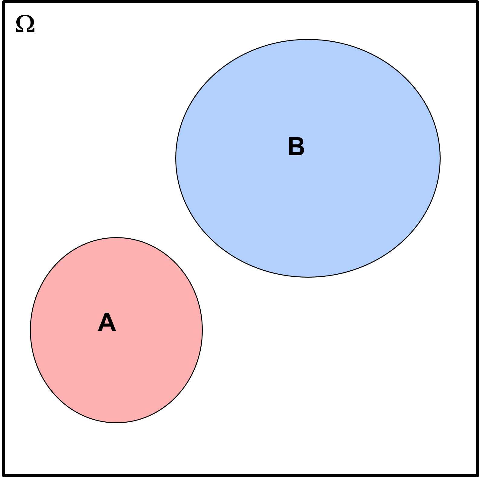
What do we learn from this Venn diagram?
the relative size of regions for each event within is the relative probability of occurrence, probability of \(B\) is greater than probability of \(A\)
the overlap over events is the probability of joint occurrence, there is 0.0 probability of \(A\) and \(B\) occurring together
Let us include a more practical Venn diagram to ensure this concept is not too abstract. Here’s a Venn diagram from 3,000 core samples with interpreted facies
the events are sandstone (Sm) and mudstone (Fm)
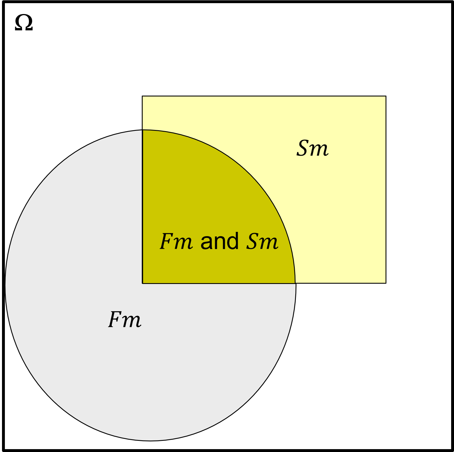
What do we learn from this Venn diagram?
mudstone is more likely than sandstone over these core samples
there are a lot of samples that are neither sandstone nor mudstone, the white space within \(\Omega\)
there are samples that are interpreted as both sandstone and mudstone, i.e., interbedded sandstone-mudstone
do not forget to draw and label the \(\Omega\) box or we can’t understand the relative probability of the events
we can use any convenient shape to represent an event
In summary, Venn diagrams are an excellent tool to visualize probability, so we will use them to visualize and teach probability here.
Frequentist Probability#
We now provide an extended definition for the frequentist approach for probability. A measure of the likelihood that an event will occur based on frequencies observed from an experiment.
For random experiments and well-defined settings, we calculate probability as:
where:
\(n(A)\) = number of times event \(A\) occurred \(n\) = number of trails
we use limit notation above to indicate sufficient sampling and that the solution converges and improves accuracy as we introduce more samples from our experiment
For example,
probability of drilling a dry hole, encountering sandstone, and exceeding a rock porosity of \(15\%\) at a location (\(\bf{u}_{\alpha}\)) based on historical results for drilling in this reservoir
Now we walk-through various probability operations from the frequentist perspective, may I ask for patience from my Bayesian friends as we will later return to the Bayesian perspective for probability.
Probability Operations#
Union of Events - for example, all outcomes in the sample space that belong to either event \(A\) or \(B\)
for the union of events operator, we use the word “or” and the mathematics symbol, \(cup\), using set notation we state the samples in the union \(A\) or \(B\) as,
and the probability notation for a union as,
Here’s a Venn diagram illustrating the union \(P(A \cup B)\).
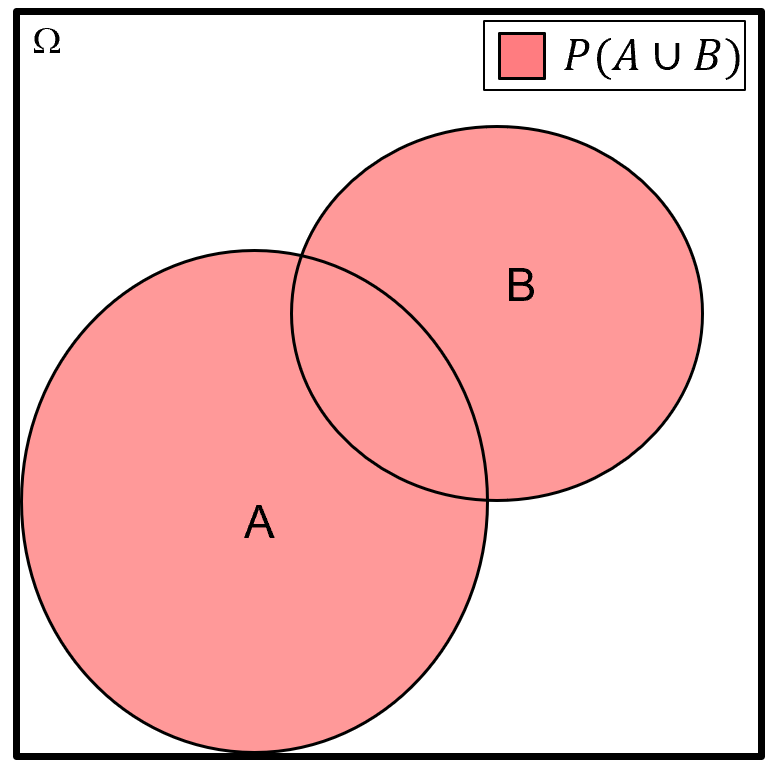
Intersection of Events - for example, all outcomes in the sample space that belong to both events \(A\) and \(B\)
for the intersection of events operator, we use the word “and” and the mathematics symbol \(cap\), using set notation we state the samples in the intersection \(A\) and \(B\) as,
and the probability notation for an intersection as,
or with the common probability shorthand as,
we will call this a joint probability later. Here is a Venn diagram illustrating the intersection \(P(A \cap B)\).
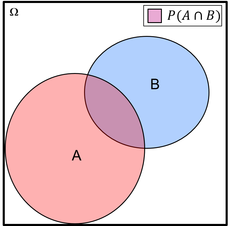
Compliment of Events - for example, all outcomes in the sample space that do not belong to event \(A\)
for the compliment of event(s) operator we use the word “not” and the mathematics symbol \(^c\), using set notation, we state the samples in the compliment of \(A\) as,
and the probability notation for a compliment as,
Here’s a Venn diagram illustrating the compliment \(P(A^c)\).
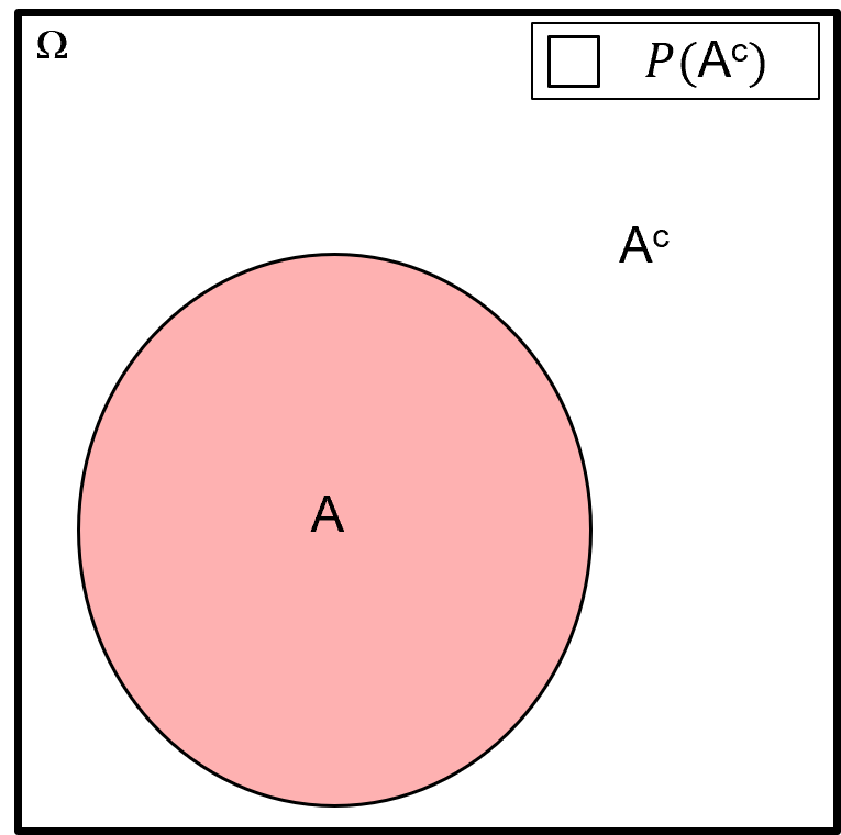
Mutually Exclusive Events - for example, events do not intersect or do not have any common outcomes, \(A\) and \(B\) do not occur at the same time.
using set notation, we state events \(A\) and \(B\) are mutually exclusive as,
and the probability notation for mutually exclusive as,
or with the common probability shorthand as,
Here’s a Venn diagram illustrating mutual exclusive events \(A\) and \(B\).

Exhaustive, Mutually Exclusive Events the sequence of events whose union is equal to the sample space, all-possible events (\(\Omega\)) and there is no intersection between the events:
using set notation, we state events \(A\) and \(B\) are exhaustive as,
and events \(A\) and \(B\) are mutually exclusive as,
and the probability notation for exhaustive events as,
and for mutually exhaustive events as,
Here’s a Venn diagram illustrating mutual exclusive, exhaustive events \(A\) and \(B\).
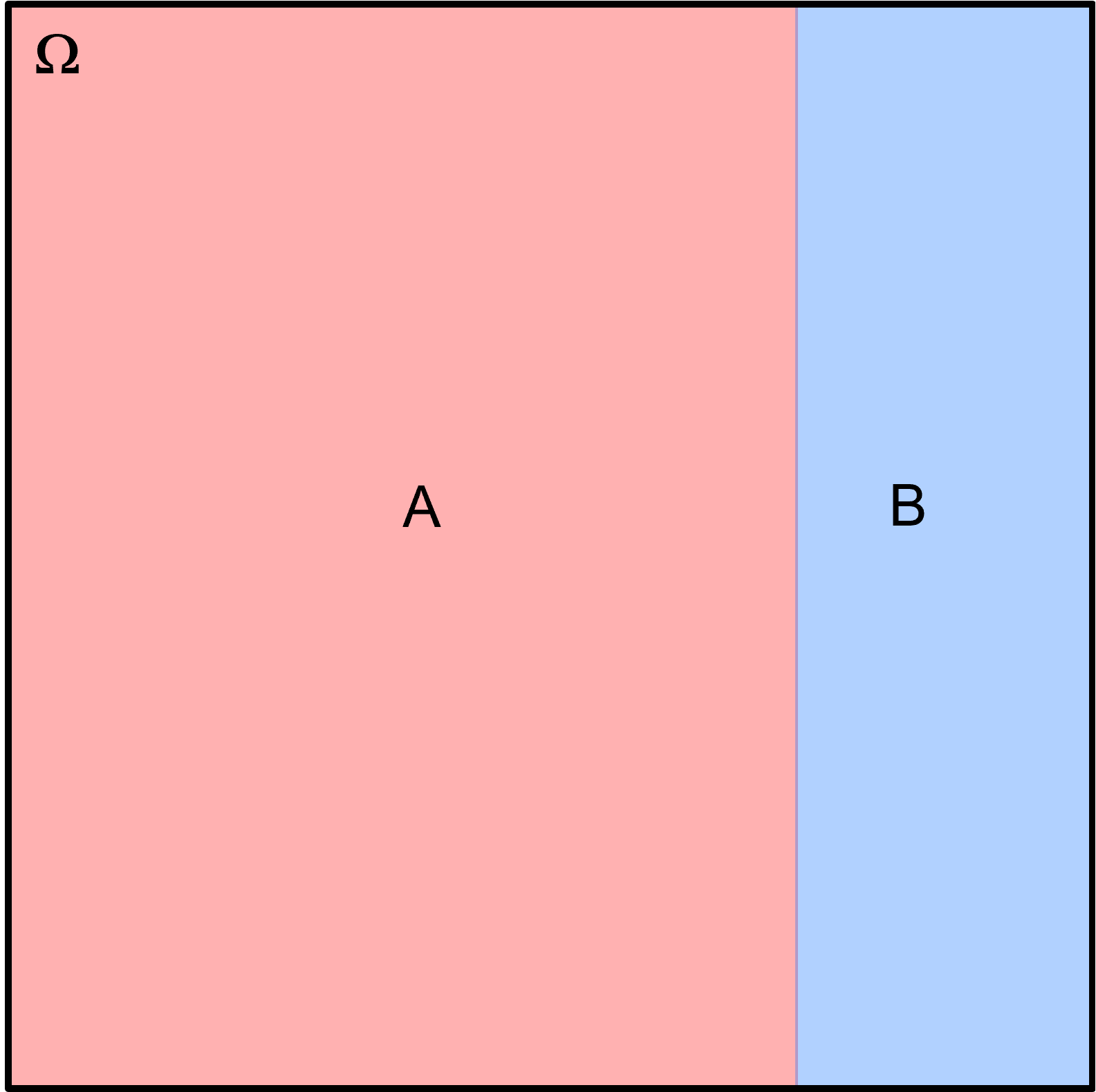
Combinations of Operators - we can use these probability operators with any number of events to communicate complicated probability cases. For example, let us define these events,
Event \(A\): oil present (\(A^c\): dry hole)
Event \(B\): 𝑆𝑚 (\(B^c\): 𝐹𝑚)
Event \(C\): porosity ≥ 15% (\(C^c\): porosity < 15%)
What is the probability of dry hole with massive sandstone (𝑆𝑚) and porosity ≥ 15%?
Here’s a Venn diagram representing this case.
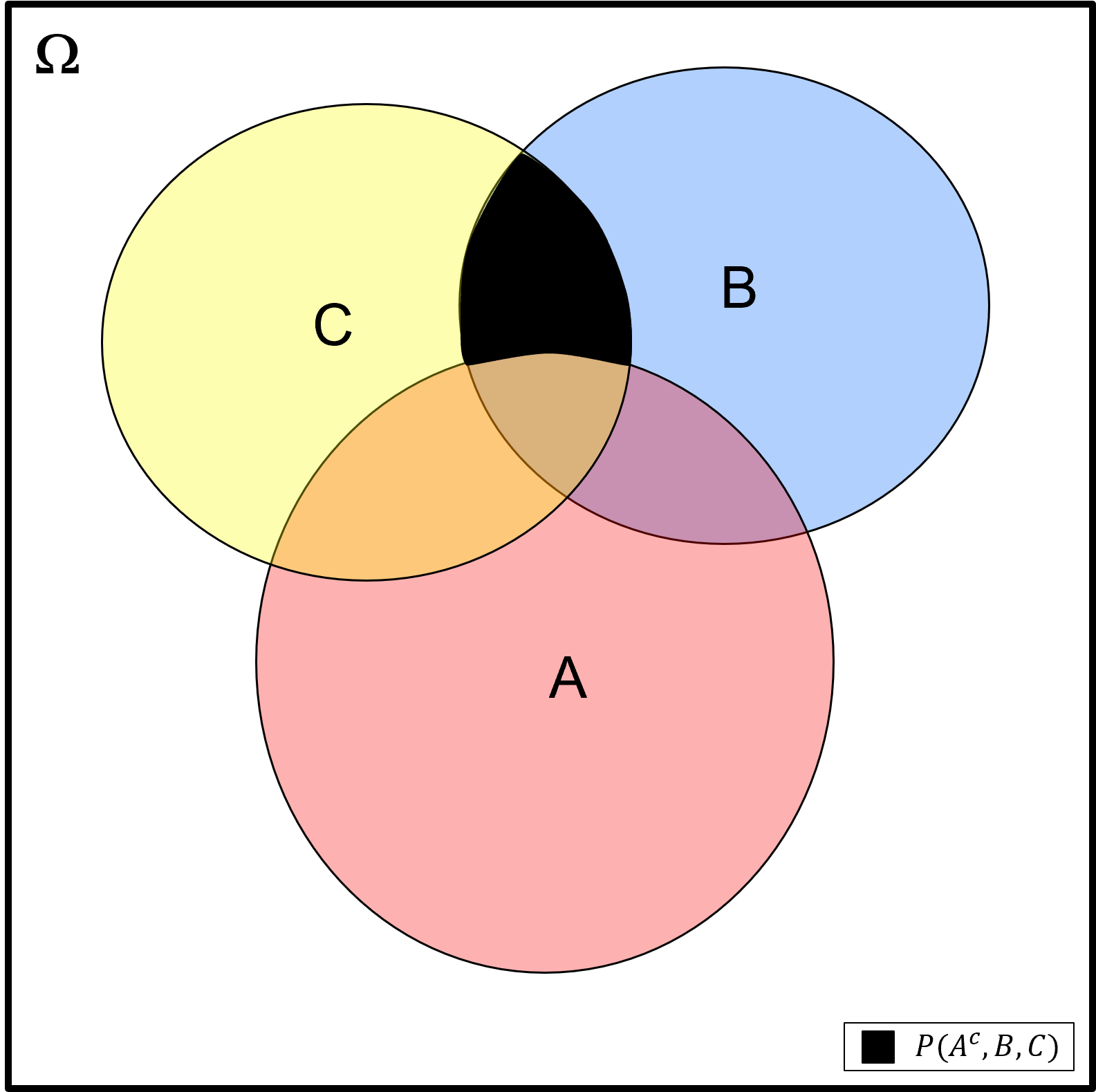
Constraints on Probability#
Now that we have defined probability notation and probability operations, now we return the idea of permissible probability values expressed by Kolmogorov. We can now build on Kolmogorov’s probability axioms with this set of probability constraints,
Non-negativity, Normalization constraints include,
Probability is bounded,
probability must be between 0.0 and 1.0 (including 0.0 and 1.0)
Probability closure,
probability of any event is 1.0
probability of A or not A is 1.0
Probability for null sets,
probability of nothing happens is zero
Now we use these probability concepts and notation to append more essential complicated probability concepts.
Probability Addition Rule#
What is the probability for a union of events? Remember that union is an “or” operation represented by the \(\cup\) notation. Consider,
inspection of the previously shown Venn diagram indicates that we can not calculate the union , \(P(A \cup B)\), by just summing \(P(A)\) and \(P(B)\).

The sum of the probabilities \(P(A)\) and \(P(B)\) will double count the intersection, \(P(A \cap B)\), so we must subtract it,
Yes, there is a general expression for any number of events to calculate the probability of the union,
I’m not going to include it here but suffice it to say that it is a book keeping nightmare given the combinatorial of intersections that can be counted too many times!
There is a much simpler case. If the events are mutually exclusive then there is no intersection, \(P(A,B) = 0.0\), and we can just sum the probabilities.
for the general case of mutually exclusive for any number of events,
then we can write this general equation for the addition rule for any number of mutually exclusive events,
Here’s a Venn diagram showing 4 mutual exclusive events, \(A_1, A_2, A_3, A_4\).
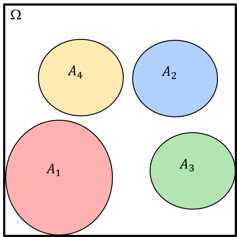
Conditional Probability#
What is the probability of an event given another event has occurred? To discuss this, let us get more specific, what is the probability of event \(B\) given event \(A\) has occurred?
to express this we use the notation, \(P(B|A)\)
we read this notation as, “probability of B given A”
This is an example of a conditional probability. We calculate conditional probability with this equation,
This may seem complicated, but we can easily visualize and understand this equation from our Venn diagram.
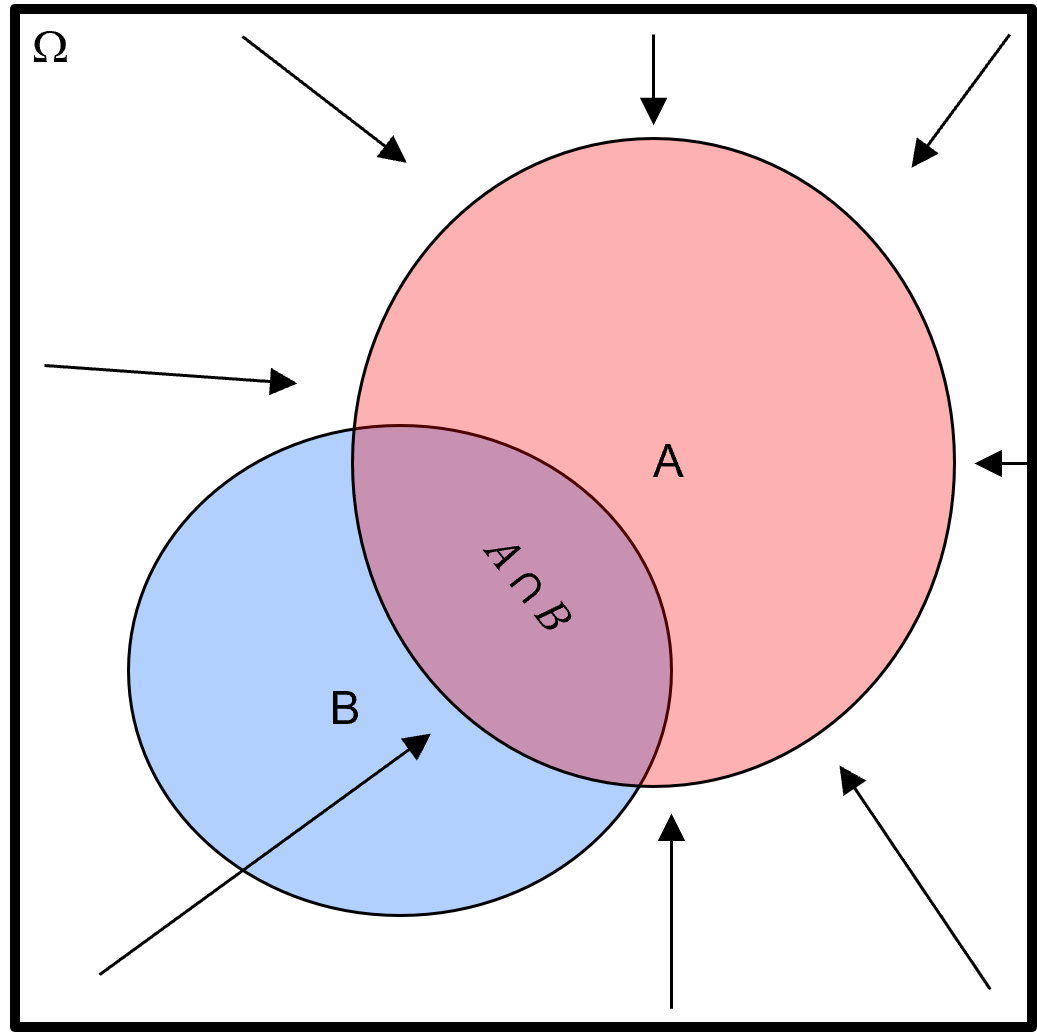
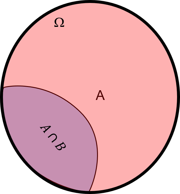
after we shrink our universe, our \(\Omega\) is only event \(A\)! Now we can easily see that the conditional probability is simply the probability of the intersection of \(A\) and \(B\) divided by the probability of \(A\).
Now we introduce a couple examples to test our knowledge of conditional probability,
Conditional Probability Example #1 - for this Venn diagram provide the conditional probabilities, \(P(A|B)\) and \(P(B|A)\), in terms of \(A\) and \(B\).
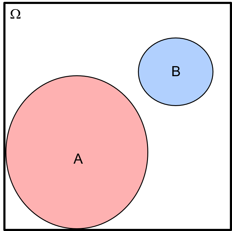
This is simple to solve, the answer is 0.0 for both conditional probability, because to calculate conditional probability the numerator is the probability, \(P(A,B)\), and this is 0.0 if there is no overlap in the Venn diagram.
also, since \(P(B,A) = P(B,A)\) the numerator is the same for both conditional probabilities,
Now we attempt a more challenging example.
Conditional Probability Example #2 - for this Venn diagram provide the conditional probabilities, \(P(A|B)\) and \(P(B|A)\), in terms of \(A\) and \(B\).
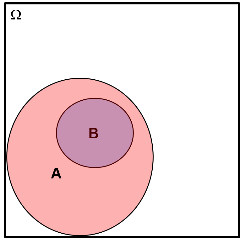
This one is more interesting. Let us look at each conditional probability one at a time.
notice that \(P(B,A) = P(B)\) since all \(B\) is inside \(A\), so we can substitute \(P(B)\) for \(P(B,A)\) above,
this makes sense, given \(B\) then \(A\) must occur, the conditional probability is 1.0. Now we calculate the other conditional probability,
just a reminder that \(P(B,A) = P(A,B)\) so we can use our previous result and substitute, \(P(B)\) for \(P(B,A)\) above.
If you understand these two examples, then you have a good foundation in conditional probability,
and I can challenge you with a more complicated without conditional probabilities and learn an interesting general case!
let us take this Venn diagram with 3 events (\(A, B, C\)) and all possible event intersections labeled.
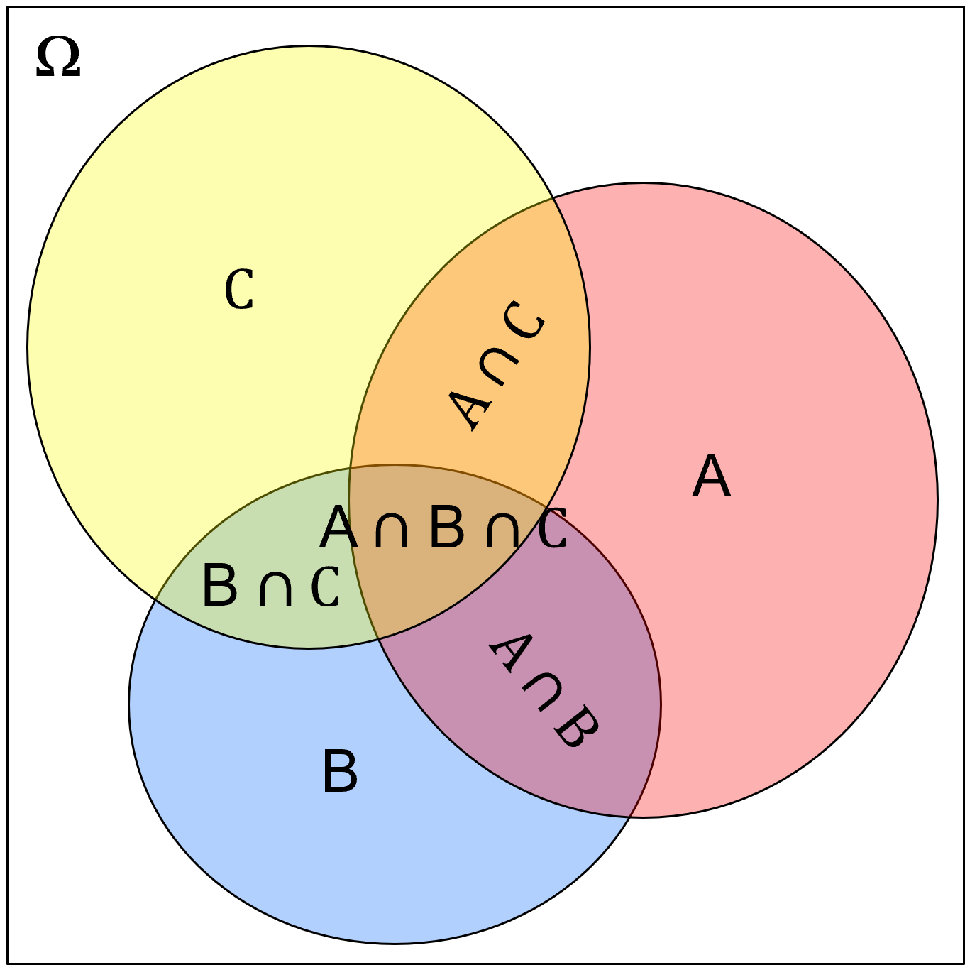
now we calculate the conditional probability,
Recalling the definition of conditional probability,
so we can reorder this to get,
spoiler alert, later we will define this at the multiplication rule, but for now we can substitute this as the denominator for the conditional probability, \(P(C|B \cap A)\), to get,
now we can reorder this as,
Do you see the pattern? We can calculate high order probability intersections as a sequential set, product sum of marginal probability and then growing conditional probabilities. Let me state it with words,
probability of \(A\), \(B\) and \(C\) is the probability of \(A\) times the probability of \(B\) given \(A\), times the probability of \(C\) given \(B\) and \(A\).
In fact, we can generalize this for any number of events as,
or more compactly,
Are we just showing off now? No! This example teaches us a lot about how conditional probabilities work.
also, this is exactly the concept used with sequential Gaussian simulation where we sample sequentially from conditional distributions instead of from the high order joint probability, an impossible task without the sequential approach!
Now we are ready to summarize marginal, conditional and joint probabilities together.
Marginal, Conditional and Joint Probabilities#
Now we define marginal, conditional and joint probability, provide notation and discuss how to calculate them:
Marginal Probability - probability of an event, irrespective of any other event,
marginal probabilities are calculated as,
marginal probabilities may be calculated from joint probabilities through the process of marginalization,
where we integrate over all cases of the other events, \(B\), to remove them.
given discrete cases of event \(B\) we can simply sum the probabilities over all cases of \(B\),
Conditional Probability - probability of an event, given another event has already occurred,
or with compaction probability notation,
see the previous section for more information, but for symmetry we repeat the method to calculate conditional probability as,
of course, as we saw in our conditional probability examples above, we cannot switch the order of the events,
Joint Probability - probability of multiple events occurring together,
or with compaction probability notation,
or even more compact as,
of course, the ordering does not matter for joint probabilities,
we calculate joint probabilities as,
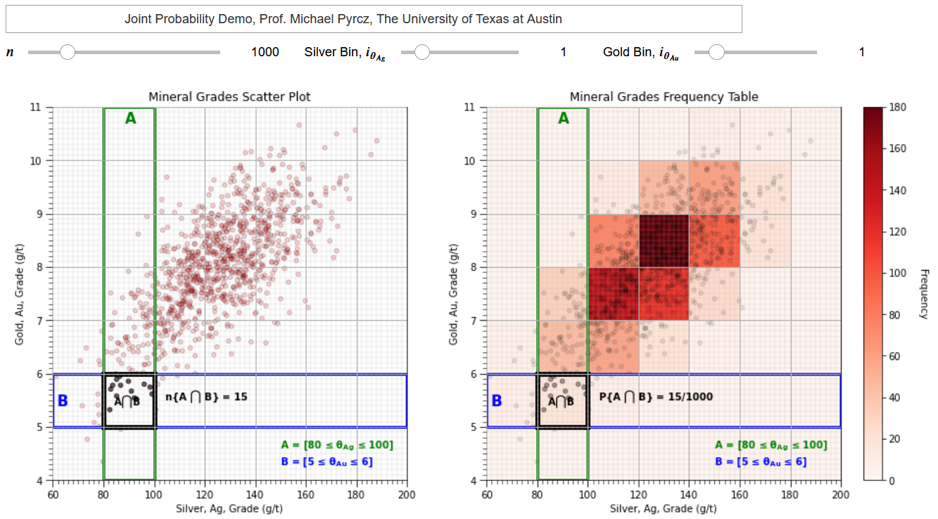
To clarify the concept of marginal, conditional and joint probability (and distributions), I have coded a set of interactive Python dashboards, Interactive_Marginal_Joint_Conditional_Probability,
that provides a dataset and interactively calculates and compares marginal, conditional and joint probabilities and visualizes and compares the marginal and conditional distributions.
Probability Multiplication Rule#
As shown above, we can calculate the joint probability of \(A\) and \(B\) as the product of the conditional probability of \(B\) given \(A\) with the marginal probability of \(A\),
and of course, we can also state,
this is know as the multiplication rule, we use the multiplication rule to develop the definition of independence.
Independent Events#
Given the probability multiplication rule,
now we ask the question, what is the conditional probability \(P(B|A)\) if events \(A\) and \(B\) are independent? Given independence between \(A\) and \(B\) we would expect that knowing about \(A\) will not impact the outcome of \(B\),
if we substitute this into \(P(A \cap B) = P(A,B) = P(B|A) \cdot P(A)\) we get,
by the same logic we can show,
Now we can summarize this as, events \(A\) and \(B\) are independent if and only if the following relations are true,
\(P(A \cap B) = P(A) \cdot P(B)\) - joint probability is the product of the marginal probabilities
\(P(A|B) = P(A)\) - conditional is the marginal probability
\(P(B|A) = P(B)\) - conditional probability is the marginal probability
If any of these are violated, we can suspect that there exists some form of relationship.
we leave the significance of this result outside the scope for this chapter on probability
certainly, if we can assume independence this simplifies our data science workflows
Independence Example #1 - check independence for the following dataset.

To check for independence, we calculate the marginal and joint probabilities,
now we check one of the conditions for independence, as the joint probability as product of the marginal probabilities,
\(P(A_1 \cap A_2) = P(A_1) \cdot P(A_2)\) \(\rightarrow\) \(0.2 \ne 0.5 \cdot 0.6\), \(\therefore\) we suspect a relationship between events \(A_1\) and \(A_2\)
Bayesian Probability#
Now we finally dive into the Bayesian approach to probability, a very flexible approach that can be applied to assign probability to anything, and includes a framework for updating with new information.
When I say that the Bayesian approach can assign probability to anything, I realize this needs some further explanation,
of course, remember my statements in the “A Warning about Calculating Probability” section above, there are times when we do not have enough data, and there are workflows that are incorrect.
I mean that any type of information can be encoded into the Bayesian framework, including belief
Let us discuss this supported by a great example from the introduction chapter of Sivia’s A Bayesian Tutorial (1996), “What is the Mass of Jupyter?”.
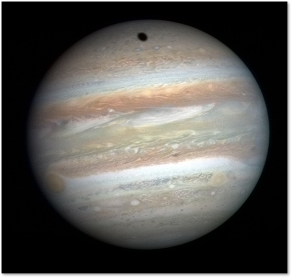
What would be frequentist and Bayesian approaches to calculate the probabilities for the uncertainty model of the mass of Jupiter?
Frequentist perspective - calculate the cumulative distribution function by measuring the mass of enough Jupiter-like planets from many star systems.
Bayesian - form a prior probability and update with any available information.
Now to anyone saying, the frequentist approach is possible, remember the first exoplanets were discovered in 1995 by astronomers Michel Mayor and Didier Queloz.
not coincidentally, the first discovered exoplanet was a Jupyter-mass hot, gas giant, as these are easier to see with the Doppler-based wobble method, because near-to-star gas giants have greater pull on their star resulting in a relatively high amplitude and frequency that can be readily observed.
when Sivia was authoring his book, there were no known exoplanets.
So, we didn’t have other Jupiter like planets to apply the frequentist approach, but we could use our knowledge about the formation of solar systems to formulate a prior model. Then we could use any available observations or measurements from Jupiter to update this prior. We could do something!
but I am getting ahead of myself, we must properly introduce the Bayesian approach to probability, by starting with Bayes’ theorem.
Bayes’ Theorem#
Once again, here’s the multiplication rule,
and it follows that we can also express it as,
If follows that,
therefore, we can substitute the right-hand sides of the multiplication rules above into this equality as,
this is Bayes’ theorem. We can make a simple modification to get the popular form of Bayes’ theorem,
To better explain Bayes’ theorem, we replace the \(A\) with “Model” and \(B\) with “New Data”, where “New Data” is the new data that we are updating with.
now we can see Bayesian updating as taking a model and updating it with new data.
Now we make some observations about Bayes’ theorem,
We are reversing conditional probabilities to get \(P(A|B)\) from \(P(B|A)\), this often comes in handy because we readily have access to one but not the other.
The probabilities in Bayes’ theorem are known as:
\(P(B)\) - evidence
\(P(A)\) - prior
\(P(B|A)\) - likelihood
\(P(A|B)\) - posterior
we can substitute the probabilities with their labels,
Prior should have no information from likelihood.
the prior probability is estimated prior to the collection of the new information in the likelihood. If the prior and likelihood includes new information, then this is “double accounting” of the new information!
Evidence term is usually just a standardization to ensure probability closure.
evidence probability is often calculated with marginalization,
for the example or two mutually exclusive, exhaustive outcomes, \(A\) and \(A^c\), then this marginalization can be applied to calculate \(P(B)\).
and by substitution we get this expanded but usually easier to calculate form of Bayes’ theorem,
we can generalize this marginalization for any number of discrete, mutually exclusive, exhaustive events as,
in some cases, like Markov chain Monte Carlo with the Metropolis-Hastings algorithm, we eliminate the need for the evidence term because we calculate a probability ratio of the proposed step vs. the current state and the evidence probability cancels out.
If the prior is naïve then the posterior is equal to the likelihood. This is logical, if we know nothing prior to collecting the new data then we completely rely on the likelihood probability.
a naïve prior is a maximum uncertainty prior, like the uniform probability with all outcomes equal probable
under the assumption of standard normal, global Gaussian distribution with a mean of 0.0 and standard deviation of 1.0, a naïve prior is the standard normal distribution
If the likelihood probability is naïve then the posterior is equal to the prior. Once again, this is logical, if the new data provides no information, then we should continue to rely on the prior probability and the original model is not updated.
Bayesian Probability Example Problems#
An efficient way to improve your understanding of Bayesian probability is through solving illustrative problems. Here’s a great group of problems,
you conduct a test and get a positive test result for something we can’t directly observe happening, but what is the probability of the thing actually happening given the positive test?
Here’s some examples of tests that fit in this class of problems,

and we can rewrite Bayes’ theorem for the case of one of these tests,

Bayesian Updating Example #1 - prior information at a site suggests a deepwater channel reservoir exists at a given location with a probability of 0.6. We consider further investigation with a 3D seismic survey.
3D seismic survey will indicate a channelized reservoir:
‐ is present with 0.9 probability if it really is present
‐ is not present with a probability 0.7 if it really is not
We have our test, seismic survey, that will offer new data, and we have our prior information (prior to collecting the new seismic data). Now we define our events,
\(A\) = the deepwater channel is present, then \(P(A)\) is the probability the thing is happening before collecting the new data
\(B\) = new seismic shows a deepwater channel, then \(P(B)\) is the probability of a positive test for the thing happening
It follows that the compliments are,
\(A^c\) = the deepwater channel not present, then \(P(A^c)\) is the probability the thing is not happening before collecting the new data
\(B^c\) = new seismic does not show a deepwater channel, then \(P(B^c)\) is the probability of a negative test for the thing happening
Now we write out Bayes’ theorem, the regular and expanded evidence term by marginalization,
What do we know? From the question above we have,
\(P(A) = 0.6\) - “prior information at a site suggests a deepwater channel reservoir exists at a given location with a probability of 0.6”
\(P(B|A) = 0.9\) - “is present with 0.9 probability if it really is present”
\(P(B^c|A^c) = 0.7\) - “is not present with a probability 0.7 if it really is not”
but we also need \(P(A^c)\) and \(P(B|A^c)\). We calculate these from closure as,
\(P(A^c) = 1.0 - P(A) = 1.0 - 0.6 = 0.4\)
\(P(B|A^c) = 1.0 - P(B^c|A^c) = 1.0 - 0.7 = 0.3\)
we have all the information that we need to substitute,
Given a positive test, seismic indicating a deepwater channel is present, we have posterior probability of 0.82.
Is seismic data useful? How do we access this?
consider the change from prior probability, 0.6, to posterior probability, 0.82, showing a reduction in uncertainty. By integrating the value and potential loss of this decision it is possible to now assign the value of information for seismic data.
I leave decision analysis out of scope for this e-book, but it is a fascinating topic, and I recommend anyone involved in data science to learn at least the basics to ensure you add value by impacting the decision(s)!
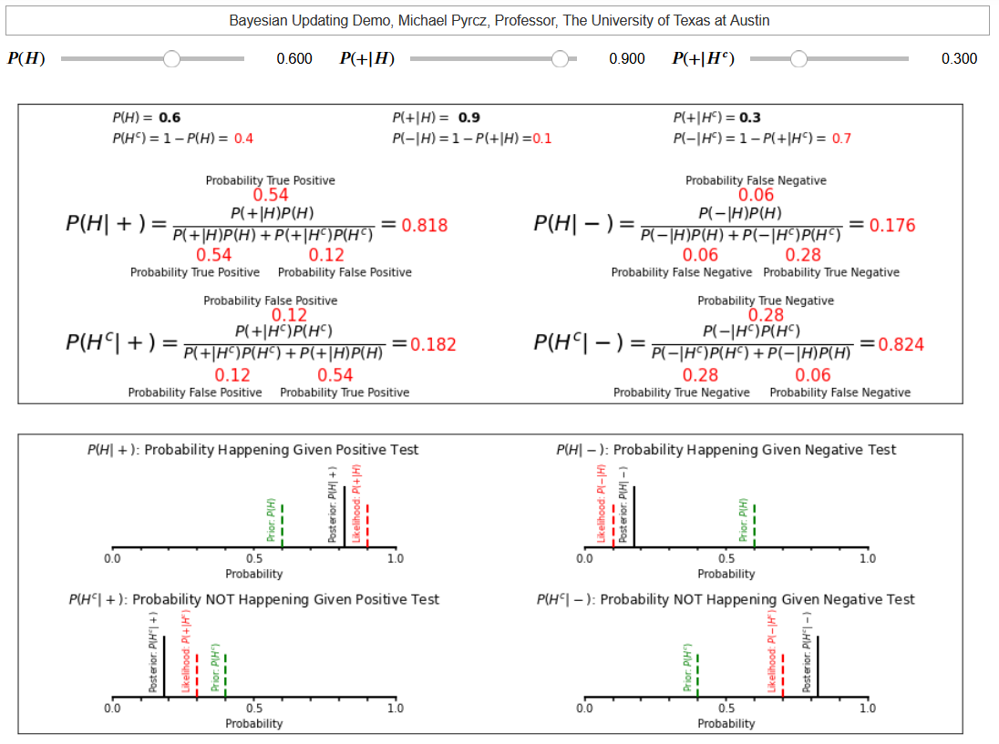
It is quite instructive to conduct a sensitivity on this example problem to assess the behavior of Bayesian updating. You could download and run my interactive Bayesian updating dashboard to accomplish this.
it is a custom dashboard to visualize Bayesian updating.

We have improved the test precision, probability of seismic detecting a channel given it is present, \(P(B|A)\) from 0.9 to 0.99.
we have almost no change in the posterior probability. Now we have improved our ability to detect no channel given the channel is not present, \(P(B|A^c)\) from 0.3 to 0.03.
we change the posterior probability from 0.82 to 0.98! What happened?
our test was being impacted by a relatively high probability of false positive, seismic showing a channel when there is no channel present, \(P(B|A^c) = 0.3\) paired with a relatively high rate of no channel present, \(P(A^c) = 0.4\).
now we switch gears and look at another illustrative example of Bayesian updating with machines on a production line.
Bayesian Updating Example #2 - You have 3 machines making the same product (imagine a large production center with 3 separate production lines working in parallel).
Each production line produces at different rates (different proportions of total production) and with different error rates (probability of an error for each unit produced).
Note we assume the products are mutually exclusive (only come from a single machine), and exhaustive (all products come from one of the 3 machines).

We want to know given an error in an individual product, what is the probability that the product came from a specific machine? First, we define our variables,
\(Y\) = the product has an error
\(X_1, X_2, X_3\) = the product came from machines 1, 2 or 3 respectively.
our Bayesian formulation for probability of defective (product with error) product coming from a specific machine is,
we will need to calculate our evidence term, P(Y) to solve this for any product. Also, we only must do this once, the evidence term is the same for all products.
We will apply marginalization to accomplish this by substituting our variables into the previously introduced general equation as,
our specific form for our problem is,
we substitute the probabilities from the problem statement as,
Given this evidence probability, now we can calculate the posterior probabilities of the product coming from each machine given the product is defective,
Let us close the loop by checking closure, we expect these posterior probabilities to sum to 1.0 over all machines (once again assuming products are mutually exclusive, and exhaustive over the machines),
and we have closure.
These two examples are very helpful to understand Bayesian updating. In the classroom I get my students to calculate the additional posteriors such as the probability of the event happening given a negative test, etc.
my second dashboard in this Jupyter notebook interactive Bayesian updating dashboard includes these examples.
I invite you to play with Bayesian updating.
Bayesian Updating with Gaussian Distributions#
Sivia (1996) provided an analytical approach for Bayesian updating under the assumption of a standard normal global distribution, Gaussian distributed with mean of 0.0 and variance of 1.0. We calculate,
the mean of the posterior distribution from the prior and likelihood mean and variance.
the variance of the posterior distribution from the prior and likelihood variances
consistent with the multivariate Gaussian distribution this posterior is homoscedastic, the prior or likelihood means are not in the equation for posterior variance.
my third dashboard in this Jupyter notebook interactive Bayesian updating dashboard includes Bayesian updating with Gaussian distributions.
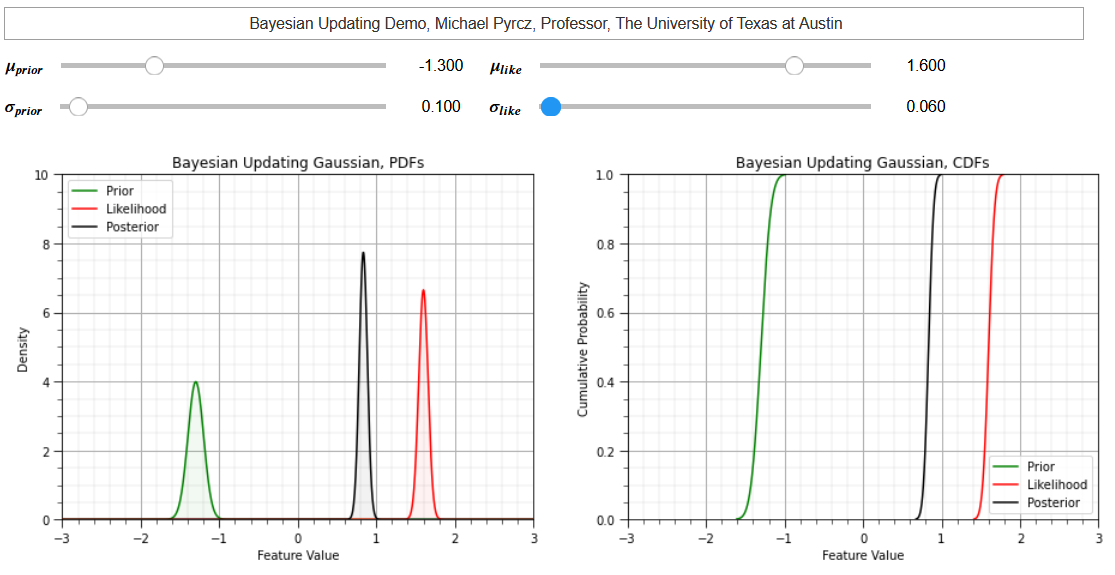
This example helps my students understand the concept of Bayesian updating for building uncertainty distributions. Here are some things to try out,
a naïve prior or likelihood and observe the posterior is the same as the likelihood or prior, respectively.
a very certain, low variance prior. Start with a large prior variance and as you reduce the variance, the posterior is pulled towards the prior. The influence of prior and likelihood is proportional to their relative certainty.
a contradiction between prior and likelihood with very different means. You may be able to even introduce extrapolation, a low prior positive mean with higher positive likelihood mean can result in an even higher positive posterior mean.
Want to Work Together?#
I hope this content is helpful to those that want to learn more about subsurface modeling, data analytics and machine learning. Students and working professionals are welcome to participate.
Want to invite me to visit your company for training, mentoring, project review, workflow design and / or consulting? I’d be happy to drop by and work with you!
Interested in partnering, supporting my graduate student research or my Subsurface Data Analytics and Machine Learning consortium (co-PIs including Profs. Foster, Torres-Verdin and van Oort)? My research combines data analytics, stochastic modeling and machine learning theory with practice to develop novel methods and workflows to add value. We are solving challenging subsurface problems!
I can be reached at mpyrcz@austin.utexas.edu.
I’m always happy to discuss,
Michael
Michael Pyrcz, Ph.D., P.Eng. Professor, Cockrell School of Engineering and The Jackson School of Geosciences, The University of Texas at Austin
More Resources Available at: Twitter | GitHub | Website | GoogleScholar | Geostatistics Book | YouTube | Applied Geostats in Python e-book | Applied Machine Learning in Python e-book | LinkedIn


Comments#
This was a basic treatment of probability. Much more could be done and discussed, I have many more resources. Check out my shared resource inventory and the YouTube lecture links at the start of this chapter with resource links in the videos’ descriptions.
I hope this is helpful,
Michael