Confidence Intervals

Confidence Intervals#

Michael J. Pyrcz, Professor, The University of Texas at Austin

Chapter of e-book “Applied Geostatistics in Python: a Hands-on Guide with GeostatsPy”.

Cite this e-Book as:

Pyrcz, M.J., 2024, Applied Geostatistics in Python: a Hands-on Guide with GeostatsPy, https://geostatsguy.github.io/GeostatsPyDemos_Book.

The workflows in this book and more are available here:

Cite the GeostatsPyDemos GitHub Repository as:

Pyrcz, M.J., 2024, GeostatsPyDemos: GeostatsPy Python Package for Spatial Data Analytics and Geostatistics Demonstration Workflows Repository (0.0.1). Zenodo. https://zenodo.org/doi/10.5281/zenodo.12667035

By Michael J. Pyrcz
© Copyright 2024.

This chapter is a tutorial for / demonstration of Confidence Intervals.

YouTube Lecture: check out my lectures on:

Motivation for Confidence Intervals#

The uncertainty in an estimated population parameter from a sample, represented as a range, lower and upper bound, based on a specified probability interval known as the confidence level.

We communicate confidence intervals like this,

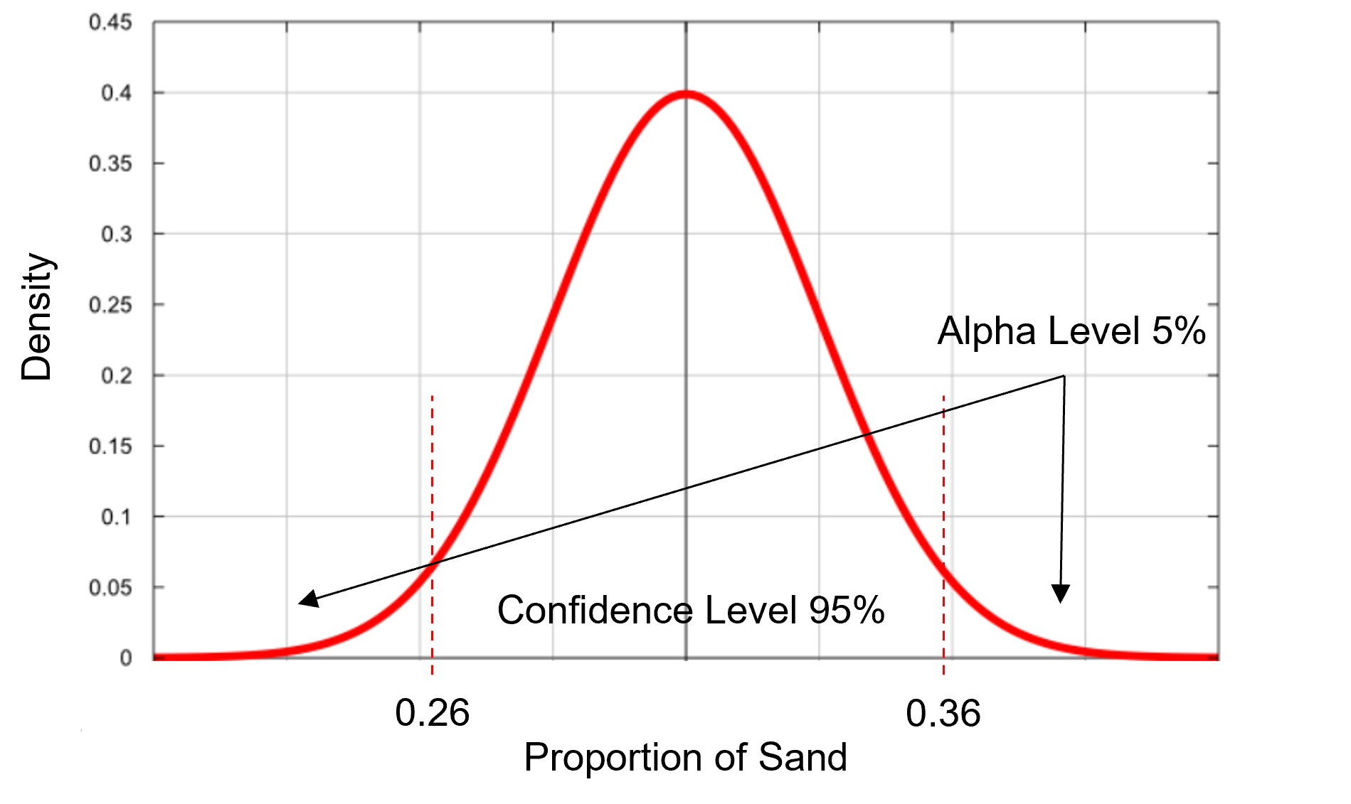
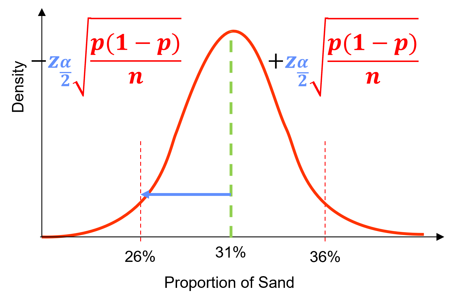
there is a 95% probability (or 19 times out of 20) that the true reservoir (population parameter), proportion of sand, is between 26% and 36%

Here we cover analytical methods for population mean and proportion,

for general bootstrap uncertainty models go to the Bootstrap Uncertainty

Confidence Level vs. Alpha Level#

To communicate confidence intervals we need to know the follow terms,

Confidence Level, the probability of the population parameter being between the assessed lower and upper confidence bounds.
Alpha level (\(\alpha\)), \(1.0 – Confidence Level\), the probability the population parameter is outside the confidence interval. Alpha level is also known as significance level.

Illustration of confidence level and alpha level for a confidence interval in the proportion of sand.

What Alpha Level (\(\alpha\)) should you use?

too wide, almost all outcomes are in the interval - not useful!
too narrow, many outcomes are outside the interval - not useful!

To determine the appropriate alpha level answer this question,

how often should a rare event occur?

The Essense of Confidence Intervals#

While our confidence interval above is communicated as,

95% probability of true reservoir proportion of sand is between 26% and 36%

We have actually calculated,

95% of sample sets with the associated confidence intervals include the true population proportion

Why is this? The confidence level refers to a long-run proportion of confidence intervals, i.e., over many samples of the confidence interval and not a specific confidence interval.

while this is not the same thing, we assume it is and move on, this is the common frequentist approach

Illustration of the actual product of confidence intervals.

Note, Bayesian credibility intervals actually represent the probablity of including the true population parameter directly in a single confidence interval.

Standard Error#

A bit of a tricky definition. Let’s start with the dictionary,

‘a measure of the statistical accuracy of an estimate, equal to the standard deviation of the theoretical distribution of a large population of such estimates’. - Oxford Dictionary

Let’s summarize,

standard error is in standard deviation, a measure of dispersion, i.e., the square root of variance
provides the uncertainty in a statistic as an estimate of the true population parameter

Now let’s show the equations for standard error, standard error in a mean:

\[ \frac{s}{\sqrt{n}} \quad \text{or} \quad \frac{s^2}{n} \]

where \(s\) is the sample standard deviation, \(s^2\) is the sample variance, and \(n\) is the number of samples. Now, the standard error in a proportion,

\[ \sqrt{\frac{\hat{p}(1-\hat{p})}{n}} \]

where \(\hat{p}\) is the sample proportion.

while we have these analytical forms, recall that we could bootstrap to solve empirically for accuracy for any statistic!
note that increasing sample variance or standard deviation increases the standard error and increasing the number of data

Scores#

Given the standard error, in standard deviation, we need to know how many standard deviations we need to include for our confidence interval to include a specific confidence level, once again we are assuming as the probability for the truth parameter to be within the interval.

the score will depend on the type of parameteric distribution, it is literally the lower and upper percentile values from the distribution
for a Gaussian distribution, we call this a z-score
for a Student’s t distribution, we call this a t-score

Analytical Confidence Interval#

We can now express confidence interval for a proportion with parts labelled as,

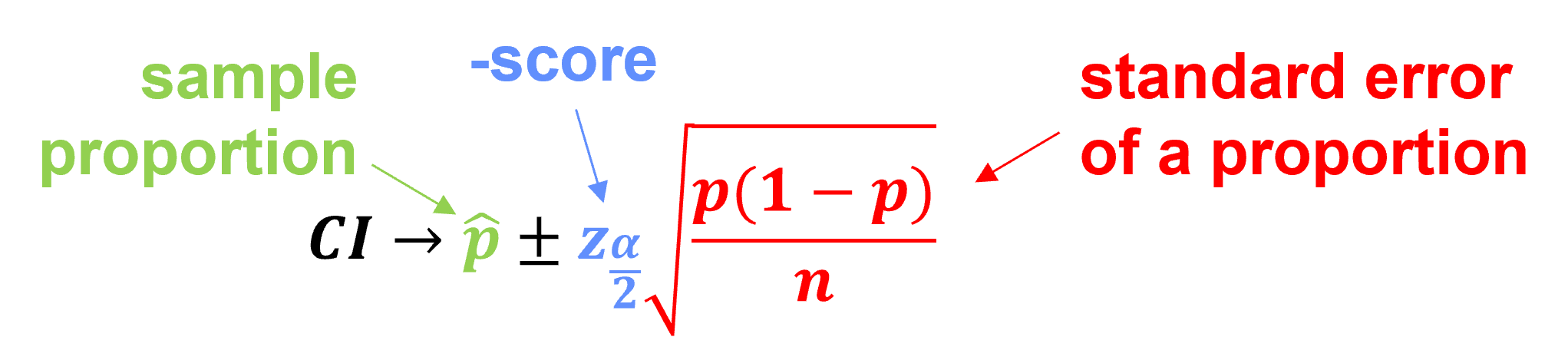
Analytical expression for confidence interval for a proportion with parts labelled.

we have a general form of,

\[ \text{Statistic} \quad \pm \quad \text{Score} \quad \times \quad \text{Standard Error} \]

and we can walk-through the calculation.

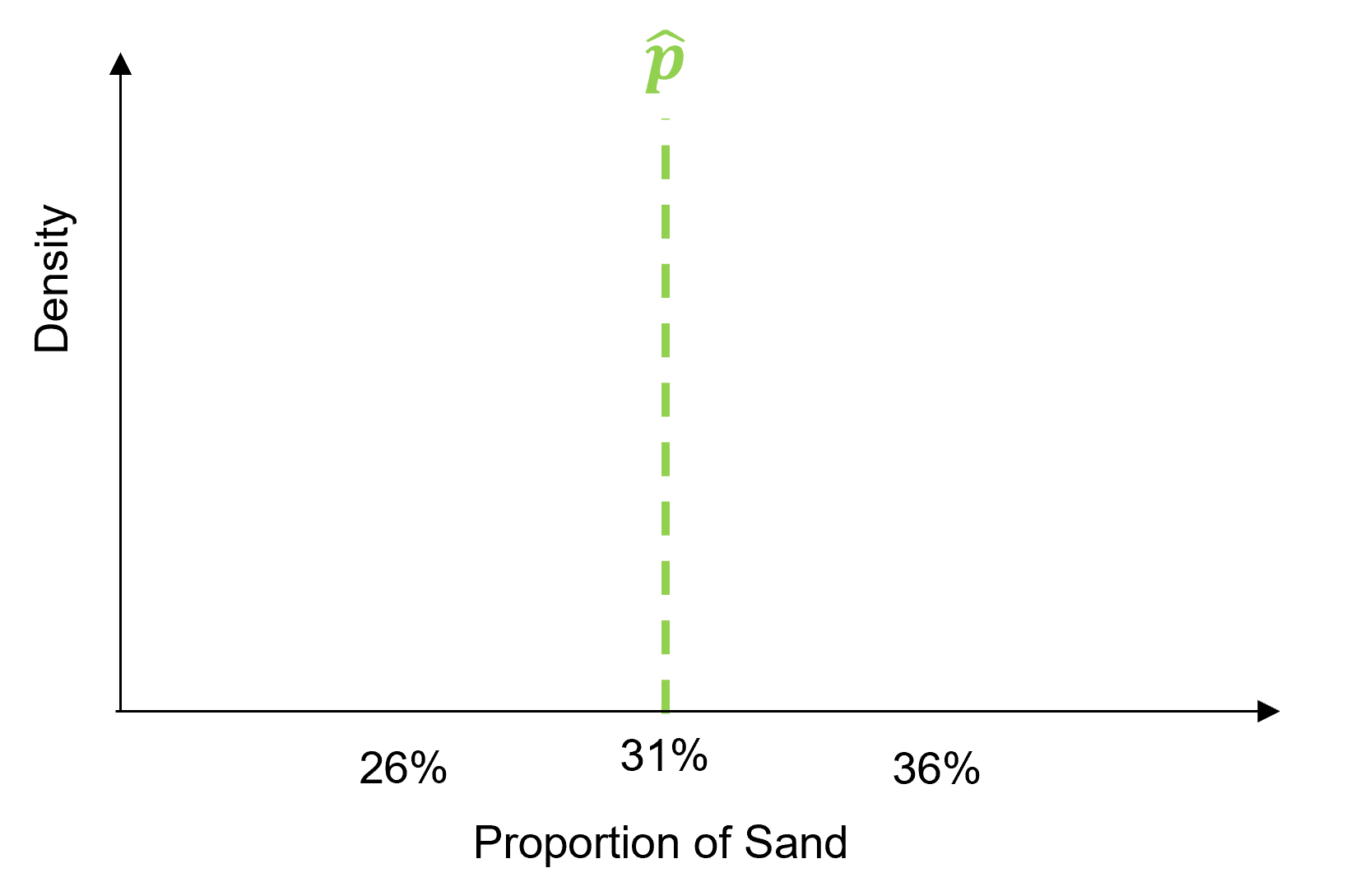
Calculate the sample Statistic, \(\hat{p}\), note, the confidence interval is centered on the statistics from the sample.

we are assuming the statistic is unbiased, the best estimate of the centroid of our uncertainty model

Our confidence interval is anchored by the available statistic.

Calculate the standard error, \(\sqrt{\frac{\hat{p}(1-\hat{p}}{n}}\), the dispersion of the uncertainty distribution in standard deviation.

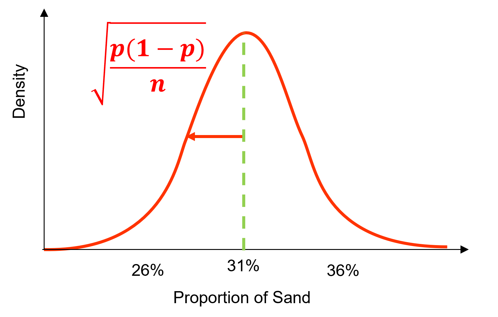
Standard error with the specific parametric distribution anchored on the sample statistic provides the entire uncertainty distribution.

Calculate the score, \(z_{\frac{\alpha}{2}}\) based on the confidence level (and alpha level).

Z-score is the symmetric percentiles from the uncertainty distribution, plus and minus centered on the sample statistic is the confidence interval.

Small Samples#

For small sample sizes our estimate of the proportion, \(p\), has additional uncertainty. We use the Student’s t distribution, with t-scores, instead of Gaussian distribution, with z-scores, to account for this.

\[ p_{C.I.} \rightarrow \hat{p} \pm z_{\frac{\alpha}{2}} \sqrt{\frac{p(1-p)}{n}} \approx \hat{p} \pm t_{\frac{\alpha}{2}} \sqrt{\frac{\hat{p}(1-\hat{p})}{n}} \]

if the sample is large then the t-score is equal to the z-score and there is no change; therefore, we could always use t-scores

What is a small sample size? There are various rules of thumb. We apply,

for means, \(n \lt 30\)
for proportions, \(np \lt 30\) or \(n(1-p) \lt 30\)

Load the Required Libraries#

The following code loads the required libraries.

import os                                                   # to set current working directory 
import numpy as np                                          # arrays and matrix math
import scipy.stats as stats                                 # statistical methods
import pandas as pd                                         # DataFrames
import math                                                 # square root
import statistics                                           # statistics
import matplotlib.pyplot as plt                             # plotting

If you get a package import error, you may have to first install some of these packages. This can usually be accomplished by opening up a command window on Windows and then typing ‘python -m pip install [package-name]’. More assistance is available with the respective package docs.

Declare Functions#

def welch_dof(x,y):                                          # DOF for Welch's test from https://pythonfordatascienceorg.wordpress.com/welch-t-test-python-pandas/
        dof = (x.var()/x.size + y.var()/y.size)**2 / ((x.var()/x.size)**2 / (x.size-1) + (y.var()/y.size)**2 / (y.size-1))
        return dof

Set the working directory#

I always like to do this so I don’t lose files and to simplify subsequent read and writes (avoid including the full address each time). Also, in this case make sure to place the required (see below) data file in this directory. When we are done with this tutorial we will write our new dataset back to this directory.

#os.chdir("C:\PGE337")                                  # set the working directory

Loading Data#

Let’s load the provided dataset. ‘PorositySamples2Units.csv’ is available at GeostatsGuy/GeoDataSets. It is a comma delimited file with 20 porosity measures from 2 rock units from the subsurface, porosity (as a fraction). We load it with the pandas ‘read_csv’ function into a data frame we called ‘df’ and then preview it by printing a slice and by utilizing the ‘head’ DataFrame member function (with a nice and clean format, see below).

#df = pd.read_csv("PorositySample2Units.csv")                # read a .csv file in as a DataFrame
df = pd.read_csv(r"https://raw.githubusercontent.com/GeostatsGuy/GeoDataSets/master/PorositySample2Units.csv") # load data from Prof. Pyrcz's github
print(df.iloc[0:5,:])                                       # display first 4 samples in the table as a preview
df.head()                                                   # we could also use this command for a table preview 

	X1	X2
0	0.21	0.20
1	0.17	0.26
2	0.15	0.20
3	0.20	0.19
4	0.19	0.13

It is useful to review the summary statistics of our loaded DataFrame. That can be accomplished with the ‘describe’ DataFrame member function. We transpose to switch the axes for ease of visualization.

df.describe().transpose()   

	count	mean	std	min	25%	50%	75%	max
X1	20.0	0.1645	0.027810	0.11	0.1500	0.17	0.19	0.21
X2	20.0	0.2000	0.045422	0.11	0.1675	0.20	0.23	0.30

Here we extract the X1 and X2 unit porosity samples from the DataFrame into separate arrays called ‘X1’ and ‘X2’ for convenience.

X1 = df['X1'].values
X2 = df['X2'].values

Confidence Interval for the Mean#

Let’s first demonstrate the calculation of the confidence interval for the sample mean at a 95% confidence level. This could be interpreted as the interval over which there is a 95% confidence that it contains the true population. We use the student’s t distribution as we assume we do not know the variance and the sample size is small.

\begin{equation} x̅ \pm t_{\frac{\alpha}{2},n-1} \times \frac {s}{\sqrt{n}} \end{equation}

ci_mean_95_x1 = stats.t.interval(0.95, len(df)-1, loc=np.mean(X1), scale=stats.sem(X1))
print('The confidence interval for the X1 mean is ' + str(np.round(ci_mean_95_x1,3)))

The confidence interval for the X1 mean is [0.151 0.178]

Confidence Interval for the Mean By-Hand#

Let’s not use the interval function and do each part by-hand.

smean = np.mean(X1); sstdev = np.std(X1); n = len(X1)
dof = len(df)-1
tscore = stats.t.ppf([0.025,0.975], df = dof)
SE = sstdev/math.sqrt(n)
lower_CI,upper_CI = np.round(smean + tscore*SE,2)
print('Statistic +/- t-score x Standard Error')
print('   ' + str(np.round(smean,3)) + '  +/-   ' + str(np.round(tscore[1],2)) + '  x     ' + str(np.round(SE,5)))
print('The confidence interval by-hand for the X1 mean is ' + str(np.round([lower_CI,upper_CI],3)))

Statistic +/- t-score x Standard Error
   0.164  +/-   2.09  x     0.00606
The confidence interval by-hand for the X1 mean is [0.15 0.18]

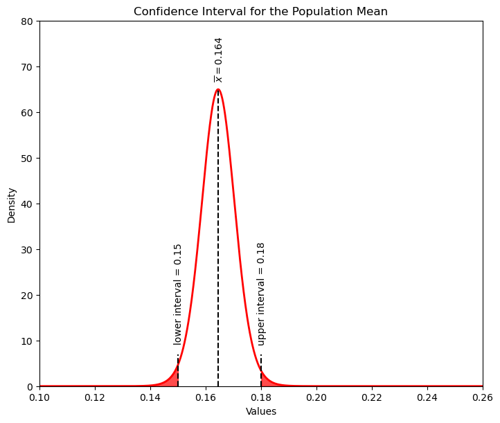
Let’s Plot the Result#

Plot the full distribution and the upper and lower confidence intervals for the uncertainty in the population mean.

xval = np.linspace(0.1,0.26,1000)
tpdf = stats.t.pdf(xval,loc=smean,df=dof,scale=SE)
plt.plot(xval,tpdf,color='red',lw=2); plt.xlabel('Values'); plt.ylabel('Density'); plt.title('Confidence Interval for the Population Mean')
plt.xlim([0.1,0.26]); plt.ylim([0,80])

plt.annotate('lower interval = ' + str(lower_CI),[lower_CI-0.0015,stats.t.pdf(lower_CI,df = dof, loc = smean, scale = sstdev/np.sqrt(n))+5],rotation=90.0)
plt.annotate('upper interval = ' + str(upper_CI),[upper_CI-0.0015,stats.t.pdf(upper_CI,df = dof, loc = smean, scale = sstdev/np.sqrt(n))+6],rotation=90.0)
plt.annotate(r'$\overline{x} = $' + str(np.round(smean,3)),[smean-0.0015,stats.t.pdf(smean,df = dof, loc = smean, scale = sstdev/np.sqrt(n))+2],rotation=90.0)
    
plt.fill_between(xval,tpdf,where= xval < lower_CI, color='red',alpha=0.7)
plt.fill_between(xval,tpdf,where= xval > upper_CI, color='red',alpha=0.7)
plt.vlines(smean,0,65,color='black',ls='--')
plt.vlines(lower_CI,0,7,color='black',ls='--'); plt.vlines(upper_CI,0,7,color='black',ls='--')

plt.subplots_adjust(left=0.0, bottom=0.0, right=1.0, top=1.1, wspace=0.3, hspace=0.4); plt.show()

_images/db6e2727aaa414c2b3fc3cbb3bcceec2ed2f94c196162a4755ae8b4836b8c8e1.png

Confidence Interval for the Proportion#

Now I demonstrate the calculation of the confidence interval for a proportion.

\begin{equation} \hat{p} \pm t_{\frac{\alpha}{2},n-1} \times \frac {\hat{p}(1-\hat{p})}{\sqrt{n}} \end{equation}

First we need to make a new categorical feature to demonstrate confidence intervals for proportions.

we will assign samples as category ‘high porosity’ when their porosity is greater than 18%

CX1 = np.where(X1 < 0.18,0,1)
prop_CX1 = np.sum(CX1 == 1)/CX1.shape[0]
print('New binary feature, 1 = high porosity, 0 = low porosity')
print(CX1)

print('\nProportion of high porosity rock in well X1 is ' + str(np.round(prop_CX1,2)))

New binary feature, 1 = high porosity, 0 = low porosity
[1 0 0 1 1 1 0 0 0 0 0 0 1 0 0 0 0 1 1 0]

Proportion of high porosity rock in well X1 is 0.35

Now we are ready to calculate the confidence interval in the proportion with the SciPy stats t interval function.

SE_prop = (prop_CX1*(1-prop_CX1))/math.sqrt(CX1.shape[0])
ci_prop_95_x1 = stats.t.interval(0.95, CX1.shape[0]-1, loc=prop_CX1, scale=SE_prop)
print('The confidence interval for the X1 proportion of high porosity is ' + str(np.round(ci_prop_95_x1,3)))

The confidence interval for the X1 proportion of high porosity is [0.244 0.456]

Confidence Interval for the Proportion By-Hand#

Let’s repeat this calculation by-hand without the SciPy stats function to test our knowledge.

sample_prop = np.sum(CX1 == 1)/CX1.shape[0]
tscore = stats.t.ppf([0.025,0.975], df = len(df)-1)
SE_prop = (prop_CX1*(1-prop_CX1))/math.sqrt(CX1.shape[0])
ci_prop_BH_95_x1 = sample_prop + tscore * SE_prop
print('Statistic +/- t-score x Standard Error')
print('   ' + str(np.round(sample_prop,3)) + '   +/-   ' + str(np.round(tscore[1],2)) + '  x     ' + str(np.round(SE_prop,4)))
print('The confidence interval for the X1 proportion of high porosity is ' + str(np.round(ci_prop_BH_95_x1,3)))

Statistic +/- t-score x Standard Error
   0.35   +/-   2.09  x     0.0509
The confidence interval for the X1 proportion of high porosity is [0.244 0.456]

Comments#

I hope you found this chapter helpful. Much more could be done and discussed, I have many more resources. Check out my shared resource inventory,

Michael

About the Author#

Michael Pyrcz is a professor in the Cockrell School of Engineering, and the Jackson School of Geosciences, at The University of Texas at Austin, where he researches and teaches subsurface, spatial data analytics, geostatistics, and machine learning. Michael is also,

the principal investigator of the Energy Analytics freshmen research initiative and a core faculty in the Machine Learn Laboratory in the College of Natural Sciences, The University of Texas at Austin
an associate editor for Computers and Geosciences, and a board member for Mathematical Geosciences, the International Association for Mathematical Geosciences.

Michael has written over 70 peer-reviewed publications, a Python package for spatial data analytics, co-authored a textbook on spatial data analytics, Geostatistical Reservoir Modeling and author of two recently released e-books, Applied Geostatistics in Python: a Hands-on Guide with GeostatsPy and Applied Machine Learning in Python: a Hands-on Guide with Code.

All of Michael’s university lectures are available on his YouTube Channel with links to 100s of Python interactive dashboards and well-documented workflows in over 40 repositories on his GitHub account, to support any interested students and working professionals with evergreen content. To find out more about Michael’s work and shared educational resources visit his Website.

Want to Work Together?#

I hope this content is helpful to those that want to learn more about subsurface modeling, data analytics and machine learning. Students and working professionals are welcome to participate.

Want to invite me to visit your company for training, mentoring, project review, workflow design and / or consulting? I’d be happy to drop by and work with you!
Interested in partnering, supporting my graduate student research or my Subsurface Data Analytics and Machine Learning consortium (co-PI is Professor John Foster)? My research combines data analytics, stochastic modeling and machine learning theory with practice to develop novel methods and workflows to add value. We are solving challenging subsurface problems!
I can be reached at mpyrcz@austin.utexas.edu.

I’m always happy to discuss,