
Kriging vs. Simulation, a 2D Map Example#
Michael J. Pyrcz, Professor, The University of Texas at Austin
Twitter | GitHub | Website | GoogleScholar | Geostatistics Book | YouTube | Applied Geostats in Python e-book | Applied Machine Learning in Python e-book | LinkedIn
Chapter of e-book “Applied Geostatistics in Python: a Hands-on Guide with GeostatsPy”.
Cite this e-Book as:
Pyrcz, M.J., 2024, Applied Geostatistics in Python: a Hands-on Guide with GeostatsPy [e-book]. Zenodo. doi:10.5281/zenodo.15169133 ![]()
The workflows in this book and more are available here:
Cite the GeostatsPyDemos GitHub Repository as:
Pyrcz, M.J., 2024, GeostatsPyDemos: GeostatsPy Python Package for Spatial Data Analytics and Geostatistics Demonstration Workflows Repository (0.0.1) [Software]. Zenodo. doi:10.5281/zenodo.12667036. GitHub Repository: GeostatsGuy/GeostatsPyDemos ![]()
By Michael J. Pyrcz
© Copyright 2024.
This chapter is a tutorial for / demonstration of Spatial Estimation with Kriging vs. Simulation with Sequential Gaussian Simulation (SGSIM) with a 2D map example.
YouTube Lecture: check out my lectures on:
For your convenience here’s a summary of the salient points.
Estimation vs. Simulation#
Let’s start by comparing spatial estimation and simulation.
Estimation:
honors local data
locally accurate, primary goal of estimation is 1 estimate!
too smooth, appropriate for visualizing trends
too smooth, inappropriate for flow simulation
one model, no assessment of global uncertainty
Simulation:
honors local data
sacrifices local accuracy, reproduces histogram
honors spatial variability, appropriate for flow simulation
alternative realizations, change random number seed
many models (realizations), assessment of global uncertainty
Spatial Estimation#
Consider the case of making an estimate at some unsampled location, \(𝑧(\bf{u}_0)\), where \(z\) is the property of interest (e.g. porosity etc.) and \(𝐮_0\) is a location vector describing the unsampled location.
How would you do this given data, \(𝑧(\bf{𝐮}_1)\), \(𝑧(\bf{𝐮}_2)\), and \(𝑧(\bf{𝐮}_3)\)?
It would be natural to use a set of linear weights to formulate the estimator given the available data.
We could add an unbiasedness constraint to impose the sum of the weights equal to one. What we will do is assign the remainder of the weight (one minus the sum of weights) to the global average; therefore, if we have no informative data we will estimate with the global average of the property of interest.
We will make a stationarity assumption, so let’s assume that we are working with residuals, \(y\).
If we substitute this form into our estimator the estimator simplifies, since the mean of the residual is zero.
while satisfying the unbiasedness constraint.
Kriging#
Now the next question is what weights should we use?
We could use equal weighting, \(\lambda = \frac{1}{n}\), and the estimator would be the average of the local data applied for the spatial estimate. This would not be very informative.
We could assign weights considering the spatial context of the data and the estimate:
spatial continuity as quantified by the variogram (and covariance function)
redundancy the degree of spatial continuity between all of the available data with themselves
closeness the degree of spatial continuity between the available data and the estimation location
The kriging approach accomplishes this, calculating the best linear unbiased weights for the local data to estimate at the unknown location. The derivation of the kriging system and the resulting linear set of equations is available in the lecture notes. Furthermore kriging provides a measure of the accuracy of the estimate! This is the kriging estimation variance (sometimes just called the kriging variance).
What is ‘best’ about this estimate? Kriging estimates are best in that they minimize the above estimation variance.
Properties of Kriging#
Here are some important properties of kriging:
Exact interpolator - kriging estimates with the data values at the data locations
Kriging variance can be calculated before getting the sample information, as the kriging estimation variance is not dependent on the values of the data nor the kriging estimate, i.e. the kriging estimator is homoscedastic.
Spatial context - kriging takes into account, furthermore to the statements on spatial continuity, closeness and redundancy we can state that kriging accounts for the configuration of the data and structural continuity of the variable being estimated.
Scale - kriging may be generalized to account for the support volume of the data and estimate. We will cover this later.
Multivariate - kriging may be generalized to account for multiple secondary data in the spatial estimate with the cokriging system. We will cover this later.
Smoothing effect of kriging can be forecast. We will use this to build stochastic simulations later.
Sequential Gaussian Simulation#
With sequential Gaussian simulation we build on kriging by:
adding a random residual with the missing variance
sequentially adding the simulated values as data to correct the covariance between the simulated values
The resulting model corrects the issues of kriging, as we now:
reproduce the global feature PDF / CDF
reproduce the global variogram
while providing a model of uncertainty through multiple realizations
In this chapter, we run kriging estimates and multiple simulation realizations, and compare the statistics.
Load the Required Libraries#
The following code loads the required libraries.
import geostatspy.GSLIB as GSLIB                              # GSLIB utilities, visualization and wrapper
import geostatspy.geostats as geostats                        # GSLIB methods convert to Python
import geostatspy
print('GeostatsPy version: ' + str(geostatspy.__version__))
GeostatsPy version: 0.0.71
We will also need some standard packages. These should have been installed with Anaconda 3.
import os                                                     # set working directory, run executables

from tqdm import tqdm                                         # suppress the status bar
from functools import partialmethod
tqdm.__init__ = partialmethod(tqdm.__init__, disable=True)

ignore_warnings = True                                        # ignore warnings?
import numpy as np                                            # ndarrays for gridded data
import pandas as pd                                           # DataFrames for tabular data
import matplotlib.pyplot as plt                               # for plotting
from matplotlib.ticker import (MultipleLocator, AutoMinorLocator) # control of axes ticks
from matplotlib import gridspec                               # custom subplots
plt.rc('axes', axisbelow=True)                                # plot all grids below the plot elements
if ignore_warnings == True:
    import warnings
    warnings.filterwarnings('ignore')
from IPython.utils import io                                  # mute output from simulation
cmap = plt.cm.inferno                                         # color map
If you get a package import error, you may have to first install some of these packages. This can usually be accomplished by opening up a command window on Windows and then typing ‘python -m pip install [package-name]’. More assistance is available with the respective package docs.
Declare Functions#
Here’s a convenience function for plotting variograms.
def vargplot(feature,lags,gamma_maj,gamma_min,npps_maj,npps_min,vmodel,azi,atol,sill,mcolor,rcolor,size,legend_pos): # plot the variogram
    index_maj,lags_maj,gmod_maj,cov_maj,ro_maj = geostats.vmodel(nlag=100,xlag=10,azm=azi,vario=vmodel);
    index_min,lags_min,gmod_min,cov_min,ro_min = geostats.vmodel(nlag=100,xlag=10,azm=azi+90.0,vario=vmodel);

    plt.scatter(lags,gamma_maj,color = 'dark'+rcolor,edgecolor = 'black',s = npps_maj*0.15*size,lw=2,
        label = 'Experimental Major', alpha = 0.8,zorder=60)
    plt.scatter(lags,gamma_min,color = rcolor,edgecolor = 'black',s = npps_min*0.10*size,lw=1,alpha = 0.8,
        label='Experimental Minor')
    plt.scatter(lags,gamma_maj,color = 'white',edgecolor = 'white',s = npps_maj*0.35*size,lw=2,
        alpha = 0.8,zorder=50)
    plt.plot(lags_maj,gmod_maj,color = 'dark'+mcolor,lw=3,label = 'Model Major',zorder=80)
    plt.plot(lags_maj,gmod_maj,color = 'white',lw=6*size,zorder=70)

    plt.plot(lags_min,gmod_min,color = mcolor,lw=1.5,label='Model Minor',zorder=60)
    plt.plot(lags_min,gmod_min,color = 'white',lw=3.0,zorder=50)
    plt.plot([0,2000],[sill,sill],color = 'black',zorder=30)
    plt.xlabel(r'Lag Distance $\bf(h)$, (m)')
    plt.ylabel(r'$\gamma \bf(h)$')
    if atol < 90.0:
        plt.title('Directional ' + feature + ' Variogram')
    else:
        plt.title('Omni Directional NSCORE ' + feature + ' Variogram')
    plt.xlim([0,1000]); plt.ylim([0,1.8*sill])
    plt.legend(loc=legend_pos)
    plt.grid(True)

def locpix_st(array,xmin,xmax,ymin,ymax,step,vmin,vmax,df,xcol,ycol,vcol,title,xlabel,ylabel,vlabel,cmap,):
    xx, yy = np.meshgrid(np.arange(xmin, xmax, step), np.arange(ymax, ymin, -1 * step))
    cs = plt.imshow(array,interpolation = None,extent = [xmin,xmax,ymin,ymax], vmin = vmin, vmax = vmax,cmap = cmap)
    plt.scatter(df[xcol],df[ycol],s=20,c=df[vcol],marker='o',cmap=cmap,vmin=vmin,vmax=vmax,alpha=0.8,linewidths=0.8,edgecolors='black',zorder=2)
    plt.scatter(df[xcol],df[ycol],s=40,c='white',marker='o',alpha=0.8,linewidths=0.8,edgecolors=None,zorder=1)
    plt.title(title); plt.xlabel(xlabel)
    plt.ylabel(ylabel); plt.xlim(xmin, xmax); plt.ylim(ymin, ymax)
    cbar = plt.colorbar(cs,orientation="vertical",cmap=cmap)
    cbar.set_label(vlabel, rotation=270, labelpad=20)
    return cs
Set the Working Directory#
I always like to do this so I don’t lose files and to simplify subsequent read and writes (avoid including the full address each time).
#os.chdir("c:/PGE383") # set the working directory
Loading Tabular Data#
Here’s the command to load our comma delimited data file in to a Pandas’ DataFrame object.
note the “fraction_data” variable is an option to random take part of the data (i.e., 1.0 is all data).
this is not standard part of spatial estimation, but fewer data is easier to visualize given our grid size (we want multiple cells between the data to see the behavior away from data)
note, I often remove unnecessary data table columns. This clarifies workflows and reduces the chance of blunders, e.g., using the wrong column!
fraction_data = 0.2                                           # extract a fraction of data for demonstration / faster runs, set to 1.0 for homework

df = pd.read_csv(r"https://raw.githubusercontent.com/GeostatsGuy/GeoDataSets/master/spatial_nonlinear_MV_facies_v1.csv")
df = df.rename(columns = {'Por':'Porosity'})                  # rename feature(s)
df = df.sample(frac = fraction_data,replace = False,random_state=13) # random sample from the dataset
df = df.reset_index()                                         # reset the record index
df = df.loc[:,['X','Y','Porosity']];                          # retain only x, y and porosity
df.head()
| X | Y | Porosity | |
|---|---|---|---|
| 0 | 390.800194 | 460.553846 | 5.774823 |
| 1 | 380.012934 | 519.379612 | 11.577469 |
| 2 | 885.824011 | 866.827752 | 13.808706 |
| 3 | 885.845177 | 355.124942 | 11.786347 |
| 4 | 855.906100 | 656.141070 | 10.422411 |
Set Limits for Plotting, Colorbars and Grid Specification#
Limits are applied for data and model visualization and the grid parameters sets the coverage and resolution of our map.
xmin = 0.0; xmax = 1000.0                                     # spatial limits
ymin = 0.0; ymax = 1000.0

nx = 100; xmn = 5.0; xsiz = 10.0                              # grid specification
ny = 100; ymn = 5.0; ysiz = 10.0

pormin = 0.0; pormax = 22.0                                   # feature limits
porvar = np.var(df['Porosity'].values)                        # assume data variance is representative

tmin = -9999.9; tmax = 9999.9                                 # triming limits
Data Analytics and Visualization#
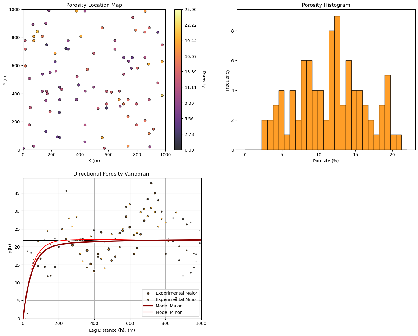
Let’s take a look at the available data:
location map
histogram
variogram
%%capture --no-display

plt.subplot(221)                                              # location map
GSLIB.locmap_st(df,'X','Y','Porosity',0,1000,0,1000,0,25,'Porosity Location Map','X (m)','Y (m)','Porosity',cmap=cmap)

plt.subplot(222)                                              # histogram
plt.hist(df['Porosity'].values,bins=np.linspace(pormin,pormax,30),color='darkorange',alpha=0.6,edgecolor='black',
         label = 'Porosity')
plt.hist(df['Porosity'].values,bins=np.linspace(pormin,pormax,30),color='darkorange',alpha=0.6,edgecolor='black',
         label = 'Porosity')
plt.xlabel('Porosity (%)'); plt.ylabel('Frequency'); plt.title('Porosity Histogram')

plt.subplot(223)                                              # variogram

lags, gamma_maj, npps_maj = geostats.gamv(df,"X","Y",'Porosity',tmin,tmax,xlag=20,xltol=20,nlag=100,azm=0.0,atol=22.5,bandwh=9999.9,isill=0);
lags, gamma_min, npps_min = geostats.gamv(df,"X","Y",'Porosity',tmin,tmax,xlag=20,xltol=20,nlag=100,azm=90.0,atol=22.5,bandwh=9999.9,isill=0);

nug = 0; nst = 2                                              # 2 nested structure variogram model parameters
it1 = 2; cc1 = 20.0; azi1 = 0; hmaj1 = 150; hmin1 = 150
it2 = 2; cc2 = 2.0; azi2 = 0; hmaj2 = 1000; hmin2 = 150

vmodel = GSLIB.make_variogram(nug,nst,it1,cc1,azi1,hmaj1,hmin1,it2,cc2,azi2,hmaj2,hmin2); # make model object
vmodel_sim = GSLIB.make_variogram(nug,nst,it1,cc1/(cc1+cc2),azi1,hmaj1,hmin1,it2,cc2/(cc1+cc2),azi2,hmaj2,hmin2); # make model object

vargplot('Porosity',lags,gamma_maj,gamma_min,npps_maj,npps_min,vmodel,azi=0.0,atol=22.5,sill=porvar,mcolor='red',rcolor='orange',size=1.0,
         legend_pos='lower right')                            # plot the variogram

plt.subplots_adjust(left=0.0, bottom=0.0, right=2.0, top=2.1, wspace=0.2, hspace=0.2); plt.show()
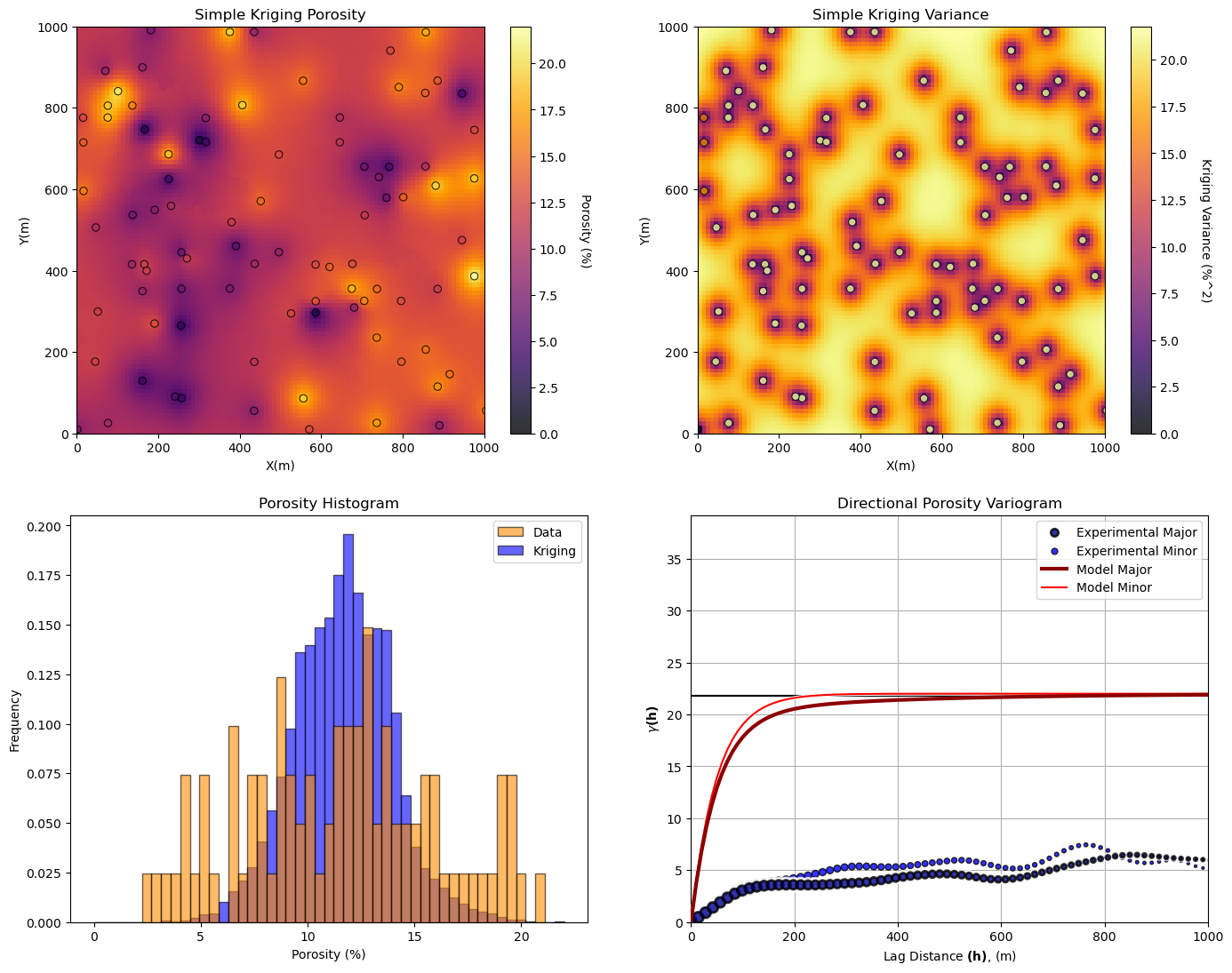
Simple Kriging#
Let’s specify the variogram model, global stationary mean and variance, and kriging parameters.
%%capture --no-display

vrange_maj = 250; vrange_min = 100                            # variogram ranges
vazi = 150.0                                                  # variogram major direction
vrel_nugget = 0.0                                             # variogram nugget effect

skmean = np.average(df['Porosity'].values)                    # assume global mean is the mean of the sample
sill = np.var(df['Porosity'].values)                          # assume sill is variance of the sample

por_vario = GSLIB.make_variogram(nug=vrel_nugget*sill,nst=1,it1=1,cc1=(1.0-vrel_nugget)*sill,
         azi1=vazi,hmaj1=vrange_maj,hmin1=vrange_min)         # porosity variogram

ktype = 0                                                     # kriging type, 0 - simple, 1 - ordinary
radius = 600                                                  # search radius for neighbouring data
nxdis = 1; nydis = 1                                          # number of grid discretizations for block kriging
ndmin = 0; ndmax = 10                                         # minimum and maximum data for an estimate
Now let’s pass this to kriging to make our porosity kriging estimate map.
%%capture --no-display

por_kmap, por_vmap = geostats.kb2d(df,'X','Y','Porosity',tmin,tmax,nx,xmn,xsiz,ny,ymn,ysiz,nxdis=1,nydis=1,
         ndmin=0,ndmax=10,radius=500,ktype=0,skmean=skmean,vario=vmodel)

plt.subplot(221)                                              # kriging estimation map
GSLIB.locpix_st(por_kmap,xmin,xmax,ymin,ymax,xsiz,pormin,pormax,df,'X','Y','Porosity','Simple Kriging Porosity',
        'X(m)','Y(m)','Porosity (%)',cmap)

plt.subplot(222)                                              # kriging variance map
GSLIB.locpix_st(por_vmap,xmin,xmax,ymin,ymax,xsiz,0,sill,df,'X','Y','X','Simple Kriging Variance','X(m)','Y(m)',
        'Kriging Variance (%^2)',cmap)

plt.subplot(223)                                              # histograms
plt.hist(df['Porosity'].values,density=True,bins=np.linspace(pormin,pormax,50),color='darkorange',alpha=0.6,
    edgecolor='black',label='Data',zorder=10)
plt.hist(por_kmap.flatten(),density=True,bins=np.linspace(pormin,pormax,50),color='blue',alpha=0.6,
    edgecolor='black',label='Kriging',zorder=1)
plt.xlabel('Porosity (%)'); plt.ylabel('Frequency'); plt.title('Porosity Histogram'); plt.legend(loc='upper right')

lags, sk_gamma_maj, npps_maj = geostats.gam(por_kmap,tmin,tmax,xsiz,ysiz,ixd=1,iyd=-1,nlag=100,isill=0.0);
lags, sk_gamma_min, npps_min = geostats.gam(por_kmap,tmin,tmax,xsiz,ysiz,ixd=1,iyd=1,nlag=100,isill=0.0);

plt.subplot(224)                                               # experimental variograms
vargplot('Porosity',lags,sk_gamma_maj,sk_gamma_min,npps_maj,npps_min,vmodel,azi=0.0,atol=22.5,sill=porvar,
         mcolor = 'red', rcolor = 'blue',size= 0.05,legend_pos = 'upper right')                # plot the variogram

plt.subplots_adjust(left=0.0, bottom=0.0, right=2.0, top=2.1, wspace=0.2, hspace=0.2); plt.show()
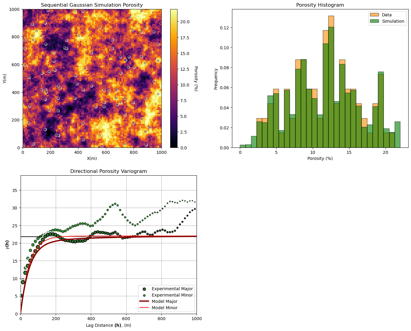
Sequential Gaussian Simulation#
Let’s jump right to building a variety of models with simulation and visualizing the results. We will start with a test, comparasion of simulation with simple and ordinary kriging.
%%capture --no-display

run = True                                                    # run the realizations, it will likely take minutes to complete

if run:
    por_sim_one = geostats.sgsim(df,'X','Y','Porosity',wcol=-1,scol=-1,tmin=tmin,tmax=tmax,itrans=1,ismooth=0,dftrans=0,tcol=0,
            twtcol=0,zmin=pormin,zmax=pormax,ltail=1,ltpar=0.0,utail=1,utpar=0.3,nsim=1,
            nx=nx,xmn=xmn,xsiz=xsiz,ny=ny,ymn=ymn,ysiz=ysiz,seed=73073,
            ndmin=0,ndmax=20,nodmax=20,mults=0,nmult=2,noct=-1,
            ktype=0,colocorr=0.0,sec_map=0,vario=vmodel_sim)[0]

plt.subplot(221)                                              # pixelplot and location map
locpix_st(por_sim_one,xmin,xmax,ymin,ymax,xsiz,pormin,pormax,df,'X','Y','Porosity','Sequential Gaussian Simulation Porosity','X(m)','Y(m)','Porosity (%)',cmap)

plt.subplot(222)                                              # histograms
plt.hist(df['Porosity'].values,density=True,bins=np.linspace(pormin,pormax,30),color='darkorange',alpha=0.6,edgecolor='black',label='Data')
plt.hist(por_sim_one.flatten(),density=True,bins=np.linspace(pormin,pormax,30),color='green',alpha=0.6,edgecolor='black',label='Simulation')
plt.xlabel('Porosity (%)'); plt.ylabel('Frequency'); plt.title('Porosity Histogram'); plt.legend(loc='upper right')

lags, sim_gamma_maj, npps_maj = geostats.gam(por_sim_one,tmin,tmax,xsiz,ysiz,ixd=1,iyd=-1,nlag=100,isill=0.0);
lags, sim_gamma_min, npps_min = geostats.gam(por_sim_one,tmin,tmax,xsiz,ysiz,ixd=1,iyd=1,nlag=100,isill=0.0);

plt.subplot(223)                                              # variograms
vargplot('Porosity',lags,sim_gamma_maj,sim_gamma_min,npps_maj,npps_min,vmodel,azi=0.0,atol=22.5,sill=porvar,
        mcolor = 'red', rcolor = 'green',size= 0.05,legend_pos = 'lower right')     # plot the variogram

plt.subplots_adjust(left=0.0, bottom=0.0, right=2.0, top=2.1, wspace=0.2, hspace=0.2); plt.show()
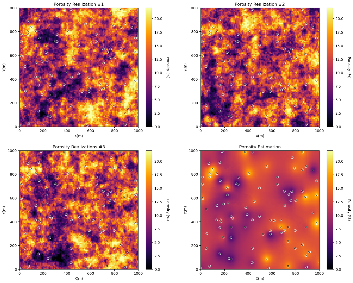
Visualize Simulated Realizations and a Kriged Estimation Model#
%%capture --no-display

run = True                                                    # run the realizations, it will likely take minutes to complete
if run:
    por_sim = geostats.sgsim(df,'X','Y','Porosity',wcol=-1,scol=-1,tmin=tmin,tmax=tmax,itrans=1,ismooth=0,dftrans=0,tcol=0,
            twtcol=0,zmin=pormin,zmax=pormax,ltail=1,ltpar=0.0,utail=1,utpar=0.3,nsim=3,
            nx=nx,xmn=xmn,xsiz=xsiz,ny=ny,ymn=ymn,ysiz=ysiz,seed=73073,
            ndmin=0,ndmax=20,nodmax=20,mults=0,nmult=2,noct=-1,
            ktype=0,colocorr=0.0,sec_map=0,vario=vmodel_sim)

plt.subplot(221)                                              # pixelplot and location map
locpix_st(por_sim[0],xmin,xmax,ymin,ymax,xsiz,pormin,pormax,df,'X','Y','Porosity','Porosity Realization #1','X(m)','Y(m)','Porosity (%)',cmap)

plt.subplot(222)                                              # pixelplot and location map
locpix_st(por_sim[1],xmin,xmax,ymin,ymax,xsiz,pormin,pormax,df,'X','Y','Porosity','Porosity Realization #2','X(m)','Y(m)','Porosity (%)',cmap)

plt.subplot(223)                                              # pixelplot and location map
locpix_st(por_sim[2],xmin,xmax,ymin,ymax,xsiz,pormin,pormax,df,'X','Y','Porosity','Porosity Realizations #3','X(m)','Y(m)','Porosity (%)',cmap)

plt.subplot(224)                                              # pixelplot and location map
locpix_st(por_kmap,xmin,xmax,ymin,ymax,xsiz,pormin,pormax,df,'X','Y','Porosity','Porosity Estimation','X(m)','Y(m)','Porosity (%)',cmap)

plt.subplots_adjust(left=0.0, bottom=0.0, right=2.0, top=2.1, wspace=0.2, hspace=0.2); plt.show()
About the Author#

Michael Pyrcz is a professor in the Cockrell School of Engineering, and the Jackson School of Geosciences, at The University of Texas at Austin, where he researches and teaches subsurface, spatial data analytics, geostatistics, and machine learning. Michael is also,
the principal investigator of the Energy Analytics freshmen research initiative and a core faculty in the Machine Learn Laboratory in the College of Natural Sciences, The University of Texas at Austin
an associate editor for Computers and Geosciences, and a board member for Mathematical Geosciences, the International Association for Mathematical Geosciences.
Michael has written over 70 peer-reviewed publications, a Python package for spatial data analytics, co-authored a textbook on spatial data analytics, Geostatistical Reservoir Modeling and author of two recently released e-books, Applied Geostatistics in Python: a Hands-on Guide with GeostatsPy and Applied Machine Learning in Python: a Hands-on Guide with Code.
All of Michael’s university lectures are available on his YouTube Channel with links to 100s of Python interactive dashboards and well-documented workflows in over 40 repositories on his GitHub account, to support any interested students and working professionals with evergreen content. To find out more about Michael’s work and shared educational resources visit his Website.
Want to Work Together?#
I hope this content is helpful to those that want to learn more about subsurface modeling, data analytics and machine learning. Students and working professionals are welcome to participate.
Want to invite me to visit your company for training, mentoring, project review, workflow design and / or consulting? I’d be happy to drop by and work with you!
Interested in partnering, supporting my graduate student research or my Subsurface Data Analytics and Machine Learning consortium (co-PI is Professor John Foster)? My research combines data analytics, stochastic modeling and machine learning theory with practice to develop novel methods and workflows to add value. We are solving challenging subsurface problems!
I can be reached at mpyrcz@austin.utexas.edu.
I’m always happy to discuss,
Michael
Michael Pyrcz, Ph.D., P.Eng. Professor, Cockrell School of Engineering and The Jackson School of Geosciences, The University of Texas at Austin
More Resources Available at: Twitter | GitHub | Website | GoogleScholar | Geostatistics Book | YouTube | Applied Geostats in Python e-book | Applied Machine Learning in Python e-book | LinkedIn
Comments#
This was a basic demonstration and comparison of spatial estimation vs. spatial simulation with kriging and sequential Gaussian simulation from GeostatsPy. Much more can be done, I have other demonstrations for modeling workflows with GeostatsPy in the GitHub repository GeostatsPy_Demos.
I hope this is helpful,
Michael