

Indicator Simulation#
Michael J. Pyrcz, Professor, The University of Texas at Austin
Twitter | GitHub | Website | GoogleScholar | Book | YouTube | Applied Geostats in Python e-book | LinkedIn
Chapter of e-book “Applied Geostatistics in Python: a Hands-on Guide with GeostatsPy”.
Cite this e-Book as:
Pyrcz, M.J., 2024, Applied Geostatistics in Python: a Hands-on Guide with GeostatsPy [e-book]. Zenodo. doi:10.5281/zenodo.15169133 ![]()
The workflows in this book and more are available here:
Cite the GeostatsPyDemos GitHub Repository as:
Pyrcz, M.J., 2024, GeostatsPyDemos: GeostatsPy Python Package for Spatial Data Analytics and Geostatistics Demonstration Workflows Repository (0.0.1) [Software]. Zenodo. doi:10.5281/zenodo.12667036. GitHub Repository: GeostatsGuy/GeostatsPyDemos ![]()
By Michael J. Pyrcz
© Copyright 2024.
This chapter is a tutorial for / demonstration of Categorical Indicator Simulation with GeostatsPy for estimating spatial categorical features, e.g., like facies.
specifically we use kriging to make estimates on a grid to display as a map.
YouTube Lecture: check out my lectures on:
For your convenience here’s a summary of salient points.
Kriging is the geostatistical workhorse for:
Prediction away from wells, e.g. pre-sample assessments, interpolation and extrapolation.
Spatial cross validation.
Spatial uncertainty modeling.
First let’s explain the concept of spatial estimation.
Spatial Estimation#
Consider the case of making an estimate at some unsampled location, \(𝑧(\bf{u}_0)\), where \(z\) is the property of interest (e.g. porosity etc.) and \(𝐮_0\) is a location vector describing the unsampled location.
How would you do this given data, \(𝑧(\bf{𝐮}_1)\), \(𝑧(\bf{𝐮}_2)\), and \(𝑧(\bf{𝐮}_3)\)?
It would be natural to use a set of linear weights to formulate the estimator given the available data.
We could add an unbiasedness constraint to impose the sum of the weights equal to one. What we will do is assign the remainder of the weight (one minus the sum of weights) to the global average; therefore, if we have no informative data we will estimate with the global average of the property of interest.
We will make a stationarity assumption, so let’s assume that we are working with residuals, \(y\).
If we substitute this form into our estimator the estimator simplifies, since the mean of the residual is zero.
while satisfying the unbiasedness constraint.
Kriging#
Now the next question is what weights should we use?
We could use equal weighting, \(\lambda = \frac{1}{n}\), and the estimator would be the average of the local data applied for the spatial estimate. This would not be very informative.
We could assign weights considering the spatial context of the data and the estimate:
spatial continuity as quantified by the variogram (and covariance function)
redundancy the degree of spatial continuity between all of the available data with themselves
closeness the degree of spatial continuity between the available data and the estimation location
The kriging approach accomplishes this, calculating the best linear unbiased weights for the local data to estimate at the unknown location. The derivation of the kriging system and the resulting linear set of equations is available in the lecture notes. Furthermore kriging provides a measure of the accuracy of the estimate! This is the kriging estimation variance (sometimes just called the kriging variance).
What is ‘best’ about this estimate? Kriging estimates are best in that they minimize the above estimation variance.
Properties of Kriging#
Here are some important properties of kriging:
Exact interpolator - kriging estimates with the data values at the data locations
Kriging variance can be calculated before getting the sample information, as the kriging estimation variance is not dependent on the values of the data nor the kriging estimate, i.e. the kriging estimator is homoscedastic.
Spatial context - kriging takes into account, furthermore to the statements on spatial continuity, closeness and redundancy we can state that kriging accounts for the configuration of the data and structural continuity of the variable being estimated.
Scale - kriging may be generalized to account for the support volume of the data and estimate. We will cover this later.
Multivariate - kriging may be generalized to account for multiple secondary data in the spatial estimate with the cokriging system. We will cover this later.
Smoothing effect of kriging can be forecast. We will use this to build stochastic simulations later.
Indicator Formalism#
Here we use indicator methods to estimate a categorical feature in space, but there are many more aspects of indicator methods that we could cover:
Estimation and Simulation with categorical variables with explicit control of spatial continuity of each category
Estimation and simulation with continuous variables with explicit control of the spatial continuity of different magnitudes
Requires indicator coding of data, a probability coding based on category or threshold
Requires indicator variograms to describe the spatial continuity.
If \(i(\bf{u}:z_k)\) is an indicator for a categorical variable,
what is the probability of a realization equal to a category?
for example,
given threshold, \(z_2 = 2\), and data at \(\bf{u}_1\), \(z(\bf{u}_1) = 2\), then \(i(bf{u}_1; z_2) = 1\)
given threshold, \(z_1 = 1\), and a RV away from data, \(Z(\bf{u}_2)\) then is calculated as \(F^{-1}_{\bf{u}_2}(z_1)\) of the RV as \(i(\bf{u}_2; z_1) = 0.23\)
If \(i(\bf{u}:z_k)\) is an indicator for a continuous variable,
what is the probability of a realization less than or equal to a threshold?
for example,
given threshold, \(z_1 = 6\%\), and data at \(\bf{u}_1\), \(z(\bf{u}_1) = 8\%\), then \(i(\bf{u}_1; z_1) = 0\)
given threshold, \(z_4 = 18\%\), and a RV away from data, \(Z(\bf{u}_2) = N\left[\mu = 16\%,\sigma = 3\%\right]\) then \(i(\bf{u}_2; z_4) = 0.75\)
The indicator coding may be applied over an entire random function by indicator transform of all the random variables at each location.
Indicator Variogram#
Variogram’s calculated and modelled from the indicator transform of spatial data and used for indicator kriging. The indicator variogram is,
where \(i(\mathbf{u}_\alpha; z_k)\) and \(i(\mathbf{u}_\alpha + \mathbf{h}; z_k)\) are the indicator transforms for the \(z_k\) threshold at the tail location \(\mathbf{u}_\alpha\) and head location \(\mathbf{u}_\alpha + \mathbf{h}\) respectively.
for hard data the indicator transform \(i(\bf{u},z_k)\) is either 0 or 1, in which case the \(\left[ i(\mathbf{u}_\alpha; z_k) - i(\mathbf{u}_\alpha + \mathbf{h}; z_k) \right]^2\) is equal to 0 when the values at head and tail are both \(\le z_k\) (for continuous features) or \(= z_k\) (for categorical features), the same relative to the threshold, or 1 when they are different.
therefore, the indicator variogram is \(\frac{1}{2}\) the proportion of pairs that change! The indicator variogram can be related to probability of change over a lag distance, \(h\).
the sill of an indicator variogram is the indicator variance calculated as,
where \(p\) is the proportion of 1’s (or zeros as the function is symmetric over proportion)
Indicator Kriging#
The application of simple kriging to a set of indicator transforms, one for each threshold for a continuous features, or one for each category for cateogorical features, of the data to directly estimate the local uncertainty model cumulative distribution function at an unknown location, \(\bf{u}\).
The indicator kriging estimator is defined as,
where \(\lambda_\alpha(k)\) is the indicator kriging weight for data \(\alpha\) and category or threshold \(k\), \(i(\mathbf{u}_\alpha; k)\) is the \(k\) category or threshold indicator transform of the data at location \(\mathbf{u}_\alpha\) and \(p(k)\) is the global or local mean categorical probability (if a trend model is provided) or the continuous cumulative probability.
by estimating probability \(p^*_{IK}(\mathbf{u}; k)\) for each threshold or category we are directly estimating the distribution of uncertainty at an unsampled location without any distribution assumption (i.e., no Gaussian assumption)
The steps for indicator kriging are,
Establish a series of thresholds or categories:
for categorical features, the categories are given
for continuous features, the thresholds should cover the entire range of the feature with enough thresholds to represent the local distributions of uncertainty (so we can resolve the local cumulative distribution function’s)
for continuous features, the thresholds may be related to critical thresholds, e.g., environmental limits, economic thresholds.
Apply indicator transformation to the data
Calculate the indicator variogram from the indicator transformation of the data for each threshold or category
Apply indicator kriging to estimate the cumulative probability for continuous features or probability for categorical features at an unsampled location, using the indicator variogram for each threshold or category
Correct the final cumulative distribution function to be valid, this is called the order relations correction.
since each threshold’s cumulative probability is estimated by indicator kriging separately, the resulting cumulative distribution function may not be valid, i.e., non-monotonic increasing
since each category’s probability is estimated by indictor kriging separately, the probabilities may not sum to one
General comments,
a variogram model is needed for each threshold or category; therefore, a more difficult inference problem, however, there is greater flexibility as spatial continuity may vary by value, for example, greater spatial continuity for upper tail of the feature distribution
more readily integrates data of different types through soft data encoding, for example, we could assign a random variable (distribution) at data locations instead of a single value
Order Relations Correction#
Due to the separate estimation of each cumulative probability over each threshold with indicator kriging the cumulative distribution may not be valid, for example,
nonmonotonic behavior for continuous features
sum of categorical probabilities not equal to one (fail to honor probability closure)
For categorical features the order relations correction is the same as the L1 normalizer (machine learning feature transformations),
cumulative probability for each threshold \(i(\bf{u}_{\alpha};z_k)\) are divided by the sum of all the cumulative probabilities, \(\sum_{i=1}^K i(\bf{u}_{\alpha};z_i)\) to ensure they sum to 1.0
For continuous features this involves a two pass calculation that results in two possible cumulative distribution functions that are monotonic increasing that are then averaged to get the corrected result (see my lecture, Indicator Methods).
Spatial Simulation#
This method is critical for:
Prediction away from wells, e.g. pre-drill assessments, with uncertainty
Spatial uncertainty modeling.
Heterogeneity realizations ready for application to the transfer function.
Sequential Indicator Simulation#
Similar to sequential Gaussian simulation, except,
kriging type - replace simple kriging from indicator kriging
spatial continuity - calculate and model the indicator variograms for each continuous threshold or category for improved control of spatial continuity
local distribution of uncertainty - repeat the indicator kriging over all continuous thresholds or categories to estimate the entire continuous CDF or categorical PDF
distribution assumption - no distribution assumption is made, instead of just the kriging estimate and variance with the Gaussian distribution assumption, we have the entire local distribution of uncertainty from indicator kriging
These are the steps for sequential indicator simulation:
sequential calculating the local categorical CDF
simulating from the local categorical CDF my Monte Carlo simulation
sequentially adding the simulated values as data to correct the covariance between the simulated values
The resulting model corrects the limitations of estimation or specifically kriging, as we now:
reproduce the global feature categorical PDF / CDF, i.e., categorical proportions
reproduce the global indicator variograms
while providing a model of uncertainty through multiple realizations
In this workflow we run kriging estimates and multiple simulation realizations, and compare the statistics.
Load the Required libraries#
The following code loads the required libraries.
import geostatspy.GSLIB as GSLIB                              # GSLIB utilities, visualization and wrapper
import geostatspy.geostats as geostats                        # GSLIB methods convert to Python
import geostatspy
print('GeostatsPy version: ' + str(geostatspy.__version__))
GeostatsPy version: 0.0.71
We will also need some standard packages. These should have been installed with Anaconda 3.
import os                                                     # set working directory, run executables

from tqdm import tqdm                                         # suppress the status bar
from functools import partialmethod
tqdm.__init__ = partialmethod(tqdm.__init__, disable=True)

ignore_warnings = True                                        # ignore warnings?
import numpy as np                                            # ndarrays for gridded data
import pandas as pd                                           # DataFrames for tabular data
import matplotlib.pyplot as plt                               # for plotting
import matplotlib as mpl                                      # custom colorbar
from matplotlib.colors import LinearSegmentedColormap
from matplotlib.ticker import (MultipleLocator, AutoMinorLocator) # control of axes ticks
plt.rc('axes', axisbelow=True)                                # plot all grids below the plot elements
if ignore_warnings == True:
    import warnings
    warnings.filterwarnings('ignore')
cmap = plt.cm.inferno                                         # color map
If you get a package import error, you may have to first install some of these packages. This can usually be accomplished by opening up a command window on Windows and then typing ‘python -m pip install [package-name]’. More assistance is available with the respective package docs.
Define Functions#
This is a convenience function to add major and minor gridlines and a combine location map and pixelplot that has color maps and color bars to improve plot interpretability.
def add_grid():
    plt.gca().grid(True, which='major',linewidth = 1.0); plt.gca().grid(True, which='minor',linewidth = 0.2) # add y grids
    plt.gca().tick_params(which='major',length=7); plt.gca().tick_params(which='minor', length=4)
    plt.gca().xaxis.set_minor_locator(AutoMinorLocator()); plt.gca().yaxis.set_minor_locator(AutoMinorLocator()) # turn on minor ticks

def locpix_colormaps_st(array,xmin,xmax,ymin,ymax,step,vmin,vmax,df,xcol,ycol,vcol,title,xlabel,ylabel,vlabel_loc,vlabel,cmap_loc,cmap):
    xx, yy = np.meshgrid(
        np.arange(xmin, xmax, step), np.arange(ymax, ymin, -1 * step)
    )
    cs = plt.imshow(array,interpolation = None,extent = [xmin,xmax,ymin,ymax], vmin = vmin, vmax = vmax,cmap = cmap)
    plt.scatter(df[xcol],df[ycol],s=None,c=df[vcol],marker=None,cmap=cmap_loc,vmin=vmin,vmax=vmax,alpha=0.8,linewidths=0.8,
        edgecolors="black",)
    plt.title(title); plt.xlabel(xlabel); plt.ylabel(ylabel); plt.xlim(xmin, xmax); plt.ylim(ymin, ymax)
    cbar_loc = plt.colorbar(orientation="vertical",pad=0.08,ticks=[0, 1],
            format=mticker.FixedFormatter(['Shale','Sand'])); cbar_loc.set_label(vlabel_loc, rotation=270,labelpad=20)
    cbar = plt.colorbar(cs,orientation="vertical",pad=0.05); cbar.set_label(vlabel, rotation=270,labelpad=20)
    return cs
Make Custom Colorbar#
We make this colorbar to display our categorical, sand and shale facies.
cmap_facies = mpl.colors.ListedColormap(['grey','gold']) # sand and shale binary color map
cmap_facies.set_over('white'); cmap_facies.set_under('white')
cmap_facies_cont = LinearSegmentedColormap.from_list("cmap_facies_cont",["grey", "gold"],) # continuous color map variant
Set the Working Directory#
I always like to do this so I don’t lose files and to simplify subsequent read and writes (avoid including the full address each time).
#os.chdir("c:/PGE383") # set the working directory
Loading Tabular Data#
Here’s the command to load our comma delimited data file in to a Pandas’ DataFrame object.
note the “nsample” variable is an option to randomly take only nsamples from the dataset.
this is not standard part of spatial estimation, but fewer data is easier to visualize given our grid size (we want multiple cells between the data to see the behavior away from data)
note, I often remove unnecessary data table columns. This clarifies workflows and reduces the chance of blunders, e.g., using the wrong column!
nsample = 50                                                  # how many data to retain for speed and clear viz

df = pd.read_csv("https://raw.githubusercontent.com/GeostatsGuy/GeoDataSets/master/sample_data_MV_biased.csv") # load the data from Dr. Pyrcz's GitHub

df = df.sample(50,random_state = 73073)
df = df.reset_index()
df = df.iloc[:,2:6]                                           # remove unnecessary features

df_sand = pd.DataFrame.copy(df[df['Facies'] == 1]).reset_index()  # copy only 'Facies' = sand records
df_shale = pd.DataFrame.copy(df[df['Facies'] == 0]).reset_index() # copy only 'Facies' = shale records
df.head(n=3)                                                  # we could also use this command for a table preview
| X | Y | Facies | Porosity | |
|---|---|---|---|---|
| 0 | 280.0 | 409.0 | 1.0 | 0.136716 |
| 1 | 230.0 | 749.0 | 1.0 | 0.204587 |
| 2 | 300.0 | 500.0 | 1.0 | 0.159891 |
Summary Statistics#
Let’s look at summary statistics for all facies combined:
df.describe().transpose() # summary table of all facies combined DataFrame statistics
| count | mean | std | min | 25% | 50% | 75% | max | |
|---|---|---|---|---|---|---|---|---|
| X | 50.0 | 431.000000 | 260.801355 | 0.000000 | 222.500000 | 340.000000 | 680.000000 | 930.000000 |
| Y | 50.0 | 508.140000 | 276.122201 | 19.000000 | 264.000000 | 474.500000 | 729.000000 | 999.000000 |
| Facies | 50.0 | 0.580000 | 0.498569 | 0.000000 | 0.000000 | 1.000000 | 1.000000 | 1.000000 |
| Porosity | 50.0 | 0.123926 | 0.030533 | 0.062169 | 0.100742 | 0.122411 | 0.145025 | 0.204587 |
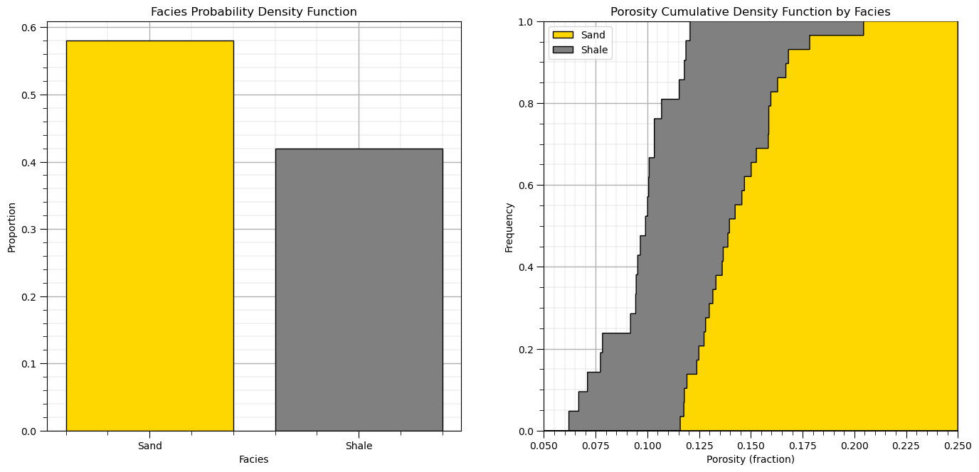
PDF and CDFs#
Let’s also look at the distributions, facies PDF and porosity CDF by facies.
plt.subplot(121)
df['Facies_Names'] = np.where(df['Facies']==0,'Shale','Sand')
facies_counts = df['Facies_Names'].value_counts()/len(df); color = ['gold','grey']
plt.bar(x=['Sand','Shale'],height=facies_counts,color=color,edgecolor='black')
plt.ylabel('Proportion'); plt.xlabel('Facies'); plt.title('Facies Probability Density Function'); add_grid()

plt.subplot(122)                                              # plot original sand and shale porosity histograms
plt.hist(df_sand['Porosity'], facecolor='gold',bins=np.linspace(0.0,0.25,1000),histtype="stepfilled",alpha=1.0,density=True,cumulative=True,edgecolor='black',label='Sand',zorder=10)
plt.hist(df_shale['Porosity'], facecolor='grey',bins=np.linspace(0.0,0.25,1000),histtype="stepfilled",alpha=1.0,density=True,cumulative=True,edgecolor='black',label='Shale',zorder=9)
plt.xlim([0.05,0.25]); plt.ylim([0,1.0])
plt.xlabel('Porosity (fraction)'); plt.ylabel('Frequency'); plt.title('Porosity')
plt.legend(loc='upper left'); plt.title('Porosity Cumulative Density Function by Facies'); add_grid()

plt.subplots_adjust(left=0.0, bottom=0.0, right=2.0, top=1.2, wspace=0.2, hspace=0.3); plt.show()
For brevity we will omit data declustering from this workflow. We will assume declustered means for the porosity and permeability to apply with simple kriging.
Specify the Grid#
Let’s specify a reasonable grid to the estimation map.
we balance detail and computation time. Note kriging computation complexity scales \(O(n_{cell})\)
so if we half the cell size we have 4 times more grid cells in 2D, 4 times the runtime
xmin = 0.0; xmax = 1000.0                                     # range of x values
ymin = 0.0; ymax = 1000.0                                     # range of y values

xsiz = 10; ysiz = 10                                          # cell size
nx = 100; ny = 100                                            # number of cells
xmn = 5; ymn = 5                                              # grid origin, location center of lower left cell

pormin = 0.05; pormax = 0.22                                  # set feature min and max for colorbars
Sequential Indicator Simulation#
Let’s jump right to building a variety of models with simulation and visualizing the results. Here we specify the simulation model parameters:
ncut - number of categories
ncut = 2                                                      # number of facies
thresh = [0,1]                                                # the facies categories (use consistent order for all lists)
gcdf = [0.4,0.6]                                              # the global proportions of the categories (shale, sand)
variomaj = 400.0; variomin = 100.0
varios = []                                                   # the variogram list
varios.append(GSLIB.make_variogram(nug=0.0,nst=1,it1=1,cc1=1.0,azi1=0,hmaj1=variomaj,hmin1=variomin)) # shale ind. vario.
varios.append(GSLIB.make_variogram(nug=0.0,nst=1,it1=1,cc1=1.0,azi1=0,hmaj1=variomaj,hmin1=variomin)) # sand ind. vario.

ndmin = 0; ndmax = 10                                         # minimum and maximum data for indicator kriging
nodmax = 10                                                   # maximum previously simulated nodes for indicator kriging
nxdis = 1; nydis = 1                                          # block kriging discretizations
dummy_trend = np.zeros((10,10))                               # current version requires trend - if wrong size = ignored
tmin = -999; tmax = 999                                       # data trimming limits
We will start with multiple realizations. We will assume a variogram and use simple indicator kriging.
we assume stationary global proportions of each facies.
%%capture --no-display

run_model = True                                              # run the simulation model
nreal = 9                                                     # number of realizations

if run_model == True:
    sim_ik = geostats.sisim(df,'X','Y','Facies',ivtype=0,koption=0,ncut=2,thresh=thresh,gcdf=gcdf,trend=dummy_trend,
               tmin=tmin,tmax=tmax,zmin=0.0,zmax=1.0,ltail=1,ltpar=1,middle=1,mpar=0,utail=1,utpar=2,
               nreal=nreal,nx=nx,xmn=xmn,xsiz=xsiz,ny=ny,ymn=ymn,ysiz=ysiz,seed = 73073,
               ndmin=ndmin,ndmax=ndmax,nodmax=nodmax,mults=1,nmult=3,noct=-1,ktype=0,vario=varios)

nrow = int(round(((nreal+0.9)/3),0))                          # adjust plot for the number of realizations
for ireal in range(0,nreal):
    plt.subplot(nrow,3,ireal+1)
    GSLIB.locpix_st(sim_ik[ireal],xmin,xmax,ymin,ymax,xsiz,-.4,1.0,df,'X','Y','Facies',
                'Sequential Indicator Simulation - Realization #' + str(ireal+1),'X(m)','Y(m)','Facies',cmap_facies)

plt.subplots_adjust(left=0.0, bottom=0.0, right=3.0, top=1.0*nrow, wspace=0.2, hspace=0.2); plt.show()
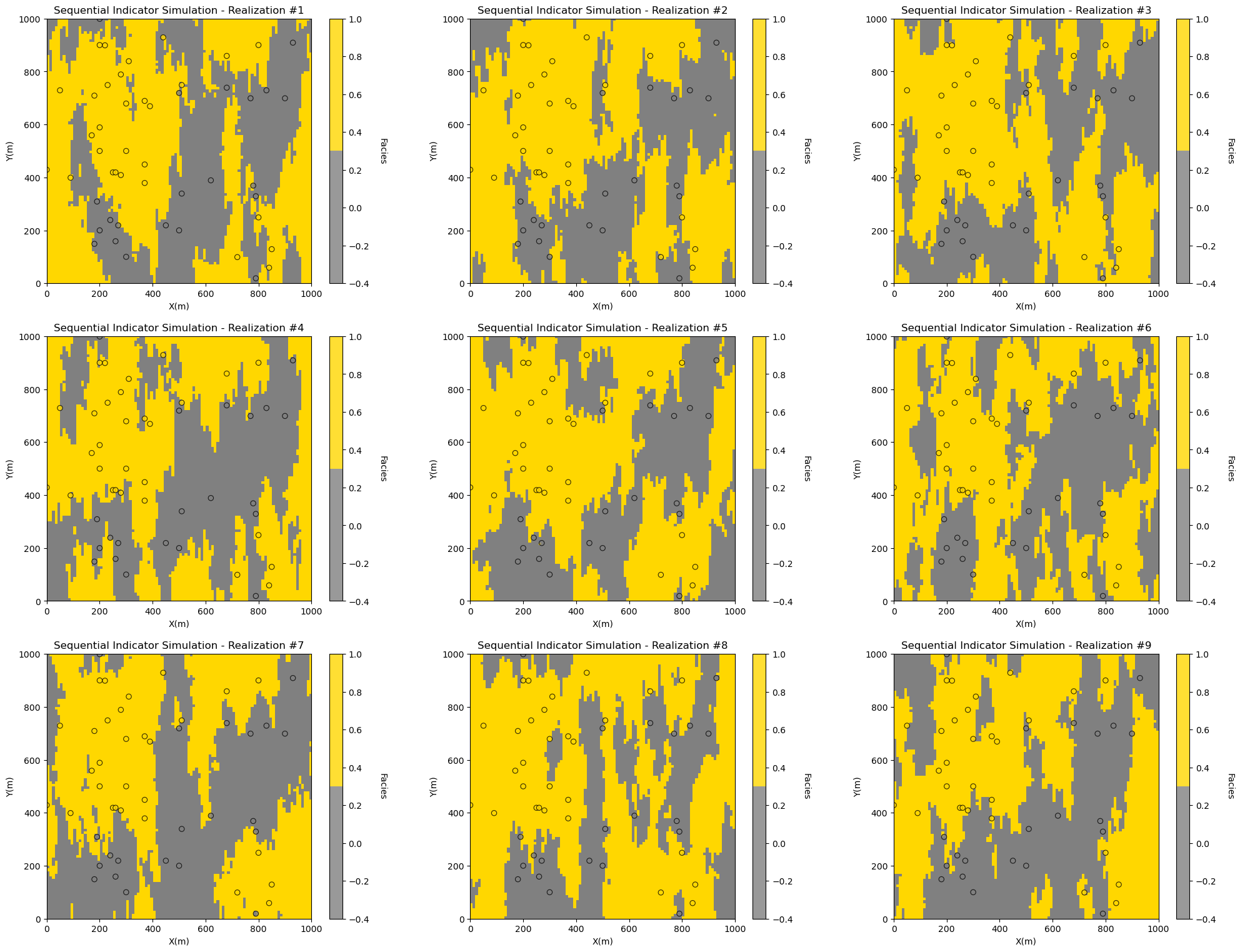
Observe the spatial continuity, relative proportions of facies and the conditioning to the available data. Let’s confirm that the representative proportions from the data are honored (the global cdf of 40% shale and 60% sand).
save = False

nrow = int(round(((nreal+0.9)/3),0))                          # adjust plot for the number of realizations
for ireal in range(0,nreal):
    plt.subplot(nrow,3,ireal+1)
    prop = [np.average(sim_ik[ireal].flatten()),1.0 - np.average(sim_ik[ireal].flatten())]; color = ['gold','grey']
    plt.bar(x=['Sand','Shale'],height=prop,color=color,edgecolor='black',label=['Real. Sand','Real. Shale'])
    plt.ylabel('Proportion'); plt.xlabel('Facies');
    plt.title('Facies Probability Density Function - Realization #' + str(ireal + 1));
    plt.scatter([0.44],[gcdf[1]],color='gold',edgecolor='black',s=100,lw=2,marker='<',zorder=20,label='Input Sand')
    plt.scatter([-0.44],[gcdf[1]],color='gold',edgecolor='black',s=100,lw=2,marker='>',zorder=20)
    plt.scatter([0.44],[gcdf[1]],color='white',s=200,lw=2,marker='<',zorder=19)
    plt.scatter([-0.44],[gcdf[1]],color='white',s=200,lw=2,marker='>',zorder=19)
    plt.scatter([1.44],[gcdf[0]],color='grey',edgecolor='black',s=100,lw=2,marker='<',zorder=20,label='Input Shale')
    plt.scatter([0.56],[gcdf[0]],color='grey',edgecolor='black',s=100,lw=2,marker='>',zorder=20)
    plt.scatter([1.44],[gcdf[0]],color='white',s=200,lw=2,marker='<',zorder=19)
    plt.scatter([0.56],[gcdf[0]],color='white',s=200,lw=2,marker='>',zorder=19)
    plt.legend(loc='upper right'); plt.ylim([0,0.8]); add_grid()

plt.subplots_adjust(left=0.0, bottom=0.0, right=3.0, top=1.0*nrow, wspace=0.2, hspace=0.2)
if save == True:
    plt.savefig('hist_Porosity_Multiple_bins.tif',dpi=600,bbox_inches="tight")
plt.show()
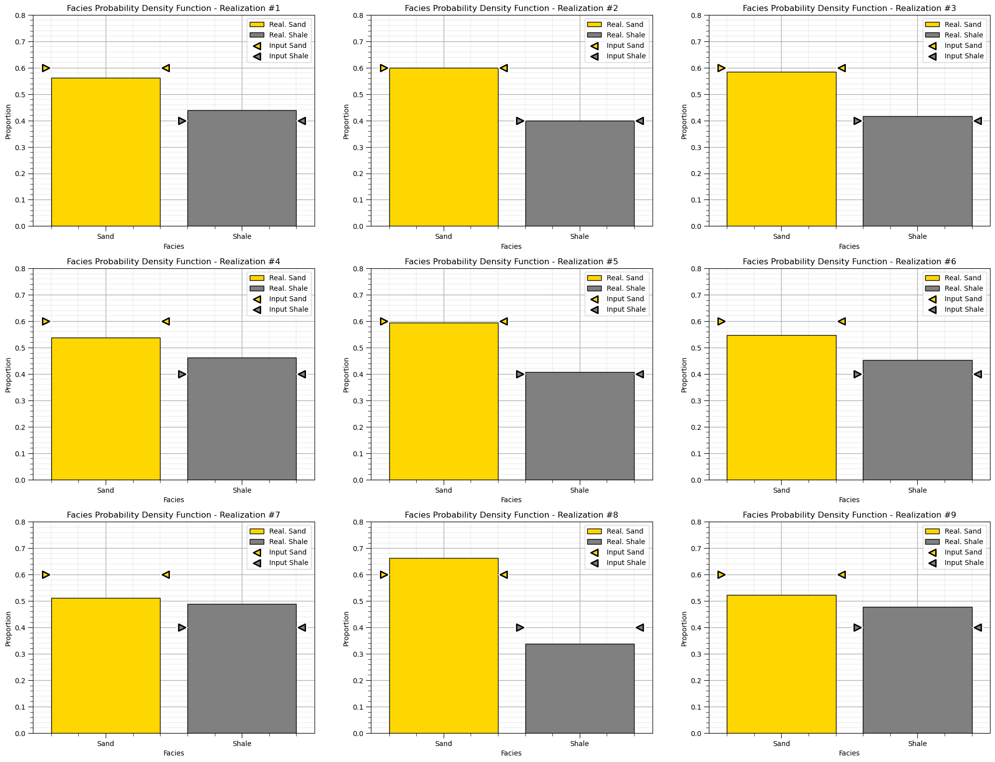
Looks good, we have some ergodic fluctuations, but that is expected.
Check the Data Conditioning#
E-type models are convenient to check data conditioning. The e-type is calculated as the average at each model cell over all the realizations.
in this case we get the proportion of sand, since sand is 1.0 and shale is 0.0
etype = np.average(sim_ik,axis=0)                     # average over axis = 0, the realizations at each node

plt.subplot(111)
GSLIB.locpix_st(etype,xmin,xmax,ymin,ymax,xsiz,0.0,1.0,df,'X','Y','Facies',
                'Sequential Indicator Simulation - E-type ','X(m)','Y(m)','Facies',cmap=cmap_facies_cont)

plt.subplots_adjust(left=0.0, bottom=0.0, right=1.0, top=1.0, wspace=0.2, hspace=0.2); plt.show()
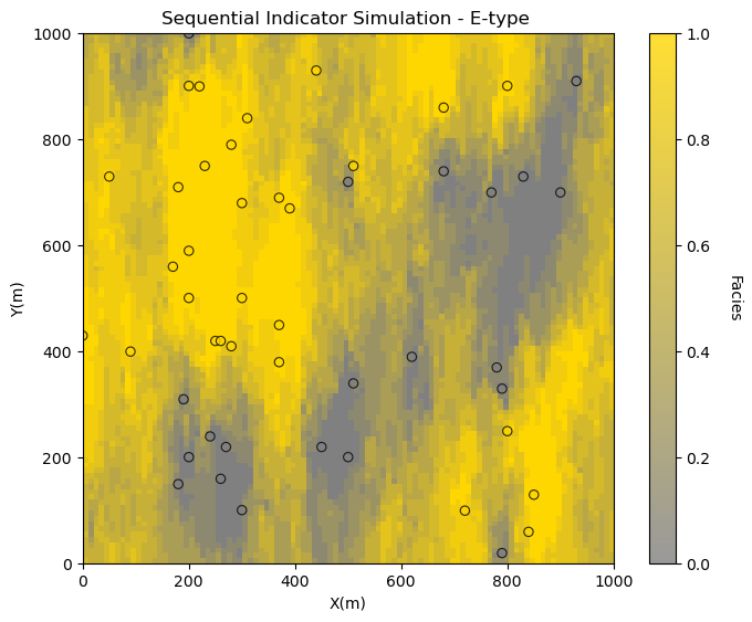
Looks like the proportion of sand is approaching 0 or 1 at the well locations, indicating that the models are conditional over the realizations.
Changing the Global Stationary Categorical Proportions#
Let’s run three realizations and significantly change the global stationary proportions and then check the results.
the global proportion is like the mean in simple kriging
as we move away from data, there is more weight on the global proportion
Let’s also shorten the variogram range to reduce the constraint of the data on the global proportion.
I also decrease the number of data and previously simulated nodes to speed up the simulation
%%capture --no-display

prop_sand = [0.5,0.6,0.7]                                      # proportion of sand cases
run_model = True                                               # run the simulation model

variomaj = 100.0; variomin = 50.0
varios = []                                                   # the variogram list
varios.append(GSLIB.make_variogram(nug=0.0,nst=1,it1=1,cc1=1.0,azi1=0,hmaj1=variomaj,hmin1=variomin)) # shale ind. vario.
varios.append(GSLIB.make_variogram(nug=0.0,nst=1,it1=1,cc1=1.0,azi1=0,hmaj1=variomaj,hmin1=variomin)) # sand ind. vario.
ndmin = 0; ndmax = 5                                          # minimum and maximum data for indicator kriging
nodmax = 5                                                    # maximum previously simulated nodes for indicator kriging

if run_model == True:
    sim_var_prop = np.zeros((len(prop_sand),ny,nx))
    for icase in range(0,len(prop_sand)):
        gcdf_var = [1.0-prop_sand[icase],prop_sand[icase]]
        sisim = geostats.sisim(df,'X','Y','Facies',ivtype=0,koption=0,ncut=2,thresh=thresh,gcdf=gcdf_var,trend=dummy_trend,
               tmin=tmin,tmax=tmax,zmin=0.0,zmax=1.0,ltail=1,ltpar=1,middle=1,mpar=0,utail=1,utpar=2,
               nreal=1,nx=nx,xmn=xmn,xsiz=xsiz,ny=ny,ymn=ymn,ysiz=ysiz,seed = 73073,
               ndmin=ndmin,ndmax=ndmax,nodmax=nodmax,mults=1,nmult=3,noct=-1,ktype=0,vario=varios)[0]
        sim_var_prop[icase] = sisim

for icase in range(0,len(prop_sand)):
    plt.subplot(len(prop_sand),2,icase*2+1)
    GSLIB.locpix_st(sim_var_prop[icase],xmin,xmax,ymin,ymax,xsiz,-.4,1.0,df,'X','Y','Facies',
                'Sequential Indicator Simulation - Input Sand Proportion ' + str(prop_sand[icase]),'X(m)','Y(m)','Facies',cmap_facies)

    plt.subplot(len(prop_sand),2,icase*2+2)
    prop = [np.average(sim_var_prop[icase].flatten()),1.0 - np.average(sim_var_prop[icase].flatten())]; color = ['gold','grey']
    plt.bar(x=['Sand','Shale'],height=prop,color=color,edgecolor='black',label=['Real. Sand','Real. Shale'])
    plt.ylabel('Proportion'); plt.xlabel('Facies');
    plt.title('Facies Probability Density Function - Realization #' + str(ireal + 1));
    plt.scatter([0.44],[gcdf[1]],color='gold',edgecolor='black',s=100,lw=2,marker='<',zorder=20,label='Input Sand')
    plt.scatter([-0.44],[gcdf[1]],color='gold',edgecolor='black',s=100,lw=2,marker='>',zorder=20)
    plt.scatter([0.44],[gcdf[1]],color='white',s=200,lw=2,marker='<',zorder=19)
    plt.scatter([-0.44],[gcdf[1]],color='white',s=200,lw=2,marker='>',zorder=19)
    plt.scatter([1.44],[gcdf[0]],color='grey',edgecolor='black',s=100,lw=2,marker='<',zorder=20,label='Input Shale')
    plt.scatter([0.56],[gcdf[0]],color='grey',edgecolor='black',s=100,lw=2,marker='>',zorder=20)
    plt.scatter([1.44],[gcdf[0]],color='white',s=200,lw=2,marker='<',zorder=19)
    plt.scatter([0.56],[gcdf[0]],color='white',s=200,lw=2,marker='>',zorder=19)
    plt.legend(loc='upper right'); plt.ylim([0,0.8]); add_grid()

plt.subplots_adjust(left=0.0, bottom=0.0, right=2.0, top=len(prop_sand), wspace=0.2, hspace=0.2); plt.show()
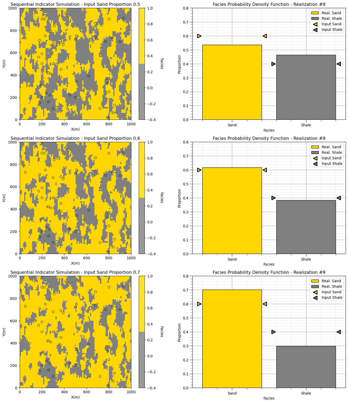
There may be a combination of ergodic fluctuations and control from the data.
if we have a high degree of spatial correlation and dense data the global proportions are constrained by the data.
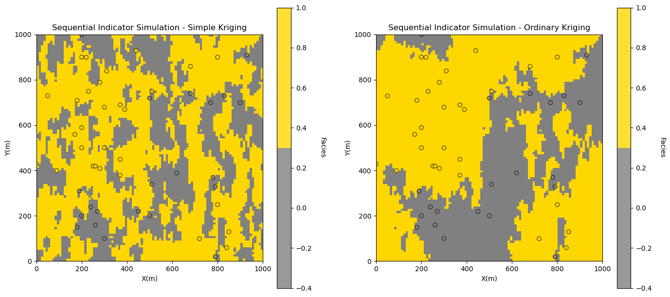
Sequential Indicator Simulation with Ordinary Kriging#
Now let’s run a realization with ordinary kriging.
relax the assumption of stationary facies proportions, by locally estimating the facies proportion.
%%capture --no-display

run_model = True                                               # run the simulation model

variomaj = 100.0; variomin = 50.0
varios = []                                                    # the variogram list
varios.append(GSLIB.make_variogram(nug=0.0,nst=1,it1=1,cc1=1.0,azi1=0,hmaj1=variomaj,hmin1=variomin)) # shale ind. vario.
varios.append(GSLIB.make_variogram(nug=0.0,nst=1,it1=1,cc1=1.0,azi1=0,hmaj1=variomaj,hmin1=variomin)) # sand ind. vario.
ndmin = 0; ndmax = 5                                           # minimum and maximum data for indicator kriging
nodmax = 5                                                     # maximum previously simulated nodes for indicator kriging


if run_model == True:
    sisim_sk = geostats.sisim(df,'X','Y','Facies',ivtype=0,koption=0,ncut=2,thresh=thresh,gcdf=gcdf,trend=dummy_trend,
               tmin=tmin,tmax=tmax,zmin=0.0,zmax=1.0,ltail=1,ltpar=1,middle=1,mpar=0,utail=1,utpar=2,
               nreal = 1,nx=nx,xmn=xmn,xsiz=xsiz,ny=ny,ymn=ymn,ysiz=ysiz,seed = 73073,
               ndmin=ndmin,ndmax=ndmax,nodmax=nodmax,mults=1,nmult=3,noct=-1,ktype=0,vario=varios)[0]

    sisim_ok = geostats.sisim(df,'X','Y','Facies',ivtype=0,koption=0,ncut=2,thresh=thresh,gcdf=gcdf,trend=dummy_trend,
               tmin=tmin,tmax=tmax,zmin=0.0,zmax=1.0,ltail=1,ltpar=1,middle=1,mpar=0,utail=1,utpar=2,
               nreal = 1,nx=nx,xmn=xmn,xsiz=xsiz,ny=ny,ymn=ymn,ysiz=ysiz,seed = 73073,
               ndmin=ndmin,ndmax=ndmax,nodmax=nodmax,mults=1,nmult=3,noct=-1,ktype=1,vario=varios)[0]


plt.subplot(121)                                               # plot the indicator simple kriging realization
GSLIB.locpix_st(sisim_sk,xmin,xmax,ymin,ymax,xsiz,-.4,1.0,df,'X','Y','Facies','Sequential Indicator Simulation - Simple Kriging',
                'X(m)','Y(m)','Facies',cmap_facies)

plt.subplot(122)                                               # plot the indicator ordinary kriging realization
GSLIB.locpix_st(sisim_ok,xmin,xmax,ymin,ymax,xsiz,-.4,1.0,df,'X','Y','Facies','Sequential Indicator Simulation - Ordinary Kriging',
                'X(m)','Y(m)','Facies',cmap_facies)

plt.subplots_adjust(left=0.0, bottom=0.0, right=2.0, top=1.2, wspace=0.2, hspace=0.2); plt.show()
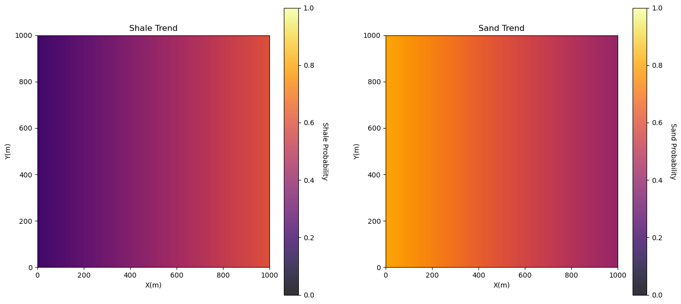
Locally Variable Proportions / Categorical Trends#
Next let’s include a trend model, also called a locally variable proportion model in the case of categorical simulation.
We will make up a simple linear trend in X for demonstration. Note with kriging option 2 and a trend model with a ndarray of dimensions [ny,nx,ncut] the program will load the local proportion to apply to 1 - sum of the weights. Note: this is not the trend / residual workflow in this first version of the program.
We make no attempt to fit a trend to the data.
Let’s just make up a trend model for demonstration. Here’s our trend.
trend = np.zeros((nx,ny,ncut)); trend[:,:,0] = 0.4; trend[:,:,1] = 0.6
for iy in range(0,ny):
    for ix in range(0,nx):
        trend[iy,ix,0] = trend[iy,ix,0] + ((ix-50)/nx) * 0.4
        trend[iy,ix,1] = trend[iy,ix,1] - ((ix-50)/nx) * 0.4

trend = geostats.correct_trend(trend)

print('Global proportion of shale = ' + str(np.average(trend[:,:,0].flatten())) )
print('Global proportion of sand = ' +  str(np.average(trend[:,:,1].flatten())) )

plt.subplot(121)
GSLIB.pixelplt_st(trend[:,:,0],xmin,xmax,ymin,ymax,xsiz,0.0,1.0,'Shale Trend','X(m)','Y(m)','Shale Probability',cmap)

plt.subplot(122)
GSLIB.pixelplt_st(trend[:,:,1],xmin,xmax,ymin,ymax,xsiz,0.0,1.0,'Sand Trend','X(m)','Y(m)','Sand Probability',cmap)

plt.subplots_adjust(left=0.0, bottom=0.0, right=2.0, top=1.2, wspace=0.2, hspace=0.2)
plt.show()
Global proportion of shale = 0.398
Global proportion of sand = 0.602
Before we run the simulation, let’s go ahead and shorted the variogram range. This will allow us to see more influence from the trend (reduce the local data constraint).
%%capture --no-display

run_model = True                                               # run the simulation model

variomaj = 50.0; variomin = 50.0
varios = []                                                    # the variogram list
varios.append(GSLIB.make_variogram(nug=0.0,nst=1,it1=1,cc1=1.0,azi1=0,hmaj1=variomaj,hmin1=variomin)) # shale ind. vario.
varios.append(GSLIB.make_variogram(nug=0.0,nst=1,it1=1,cc1=1.0,azi1=0,hmaj1=variomaj,hmin1=variomin)) # sand ind. vario.
ndmin = 0; ndmax = 5                                           # minimum and maximum data for indicator kriging
nodmax = 5                                                     # maximum previously simulated nodes for indicator kriging

if run_model == True:
    sisim_trend = geostats.sisim(df,'X','Y','Facies',ivtype=0,koption=0,ncut=2,thresh=thresh,gcdf=gcdf,trend=trend,
               tmin=tmin,tmax=tmax,zmin=0.0,zmax=1.0,ltail=1,ltpar=1,middle=1,mpar=0,utail=1,utpar=2,
               nreal=1,nx=nx,xmn=xmn,xsiz=xsiz,ny=ny,ymn=ymn,ysiz=ysiz,seed = 73073,
               ndmin=ndmin,ndmax=ndmax,nodmax=nodmax,mults=1,nmult=3,noct=-1,ktype=2,vario=varios)[0]

plt.subplot(221)
GSLIB.pixelplt_st(trend[:,:,1],xmin,xmax,ymin,ymax,xsiz,0.0,1.0,'Sand Trend','X(m)','Y(m)','Sand Probability',cmap)

plt.subplot(223)                                               # plot indicator simulation with trend
GSLIB.locpix_st(sisim_trend,xmin,xmax,ymin,ymax,xsiz,-.4,1.0,df,'X','Y','Facies',
                'Sequential Indicator Simulation - Locally Variable Proportion','X(m)','Y(m)','Facies',cmap_facies)

plt.subplot(224)
prop = [np.average(sisim_trend.flatten()),1.0 - np.average(sisim_trend.flatten())]; color = ['gold','grey']
plt.bar(x=['Sand','Shale'],height=prop,color=color,edgecolor='black',label=['Real. Sand','Real. Shale'])
plt.ylabel('Proportion'); plt.xlabel('Facies');
plt.title('Sequential Indicator Simulation - Locally Variable Proportion');
plt.scatter([0.44],[gcdf[1]],color='gold',edgecolor='black',s=100,lw=2,marker='<',zorder=20,label='Input Sand')
plt.scatter([-0.44],[gcdf[1]],color='gold',edgecolor='black',s=100,lw=2,marker='>',zorder=20)
plt.scatter([0.44],[gcdf[1]],color='white',s=200,lw=2,marker='<',zorder=19)
plt.scatter([-0.44],[gcdf[1]],color='white',s=200,lw=2,marker='>',zorder=19)
plt.scatter([1.44],[gcdf[0]],color='grey',edgecolor='black',s=100,lw=2,marker='<',zorder=20,label='Input Shale')
plt.scatter([0.56],[gcdf[0]],color='grey',edgecolor='black',s=100,lw=2,marker='>',zorder=20)
plt.scatter([1.44],[gcdf[0]],color='white',s=200,lw=2,marker='<',zorder=19)
plt.scatter([0.56],[gcdf[0]],color='white',s=200,lw=2,marker='>',zorder=19)
plt.legend(loc='upper right'); plt.ylim([0,0.8]); add_grid()

plt.subplots_adjust(left=0.0, bottom=0.0, right=2.0, top=2.1, wspace=0.2, hspace=0.2); plt.show()
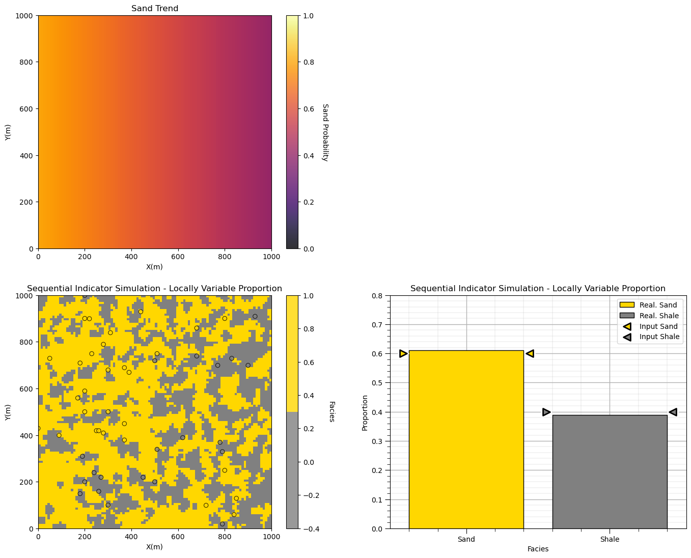
The trend is quite epic and we still match the input global proportions. We should take care to ensure that the global proportions in the trend honor the representative statistics (from declustering). The above exercise was just a simple demo.
About the Author#

Michael Pyrcz is a professor in the Cockrell School of Engineering, and the Jackson School of Geosciences, at The University of Texas at Austin, where he researches and teaches subsurface, spatial data analytics, geostatistics, and machine learning. Michael is also,
the principal investigator of the Energy Analytics freshmen research initiative and a core faculty in the Machine Learn Laboratory in the College of Natural Sciences, The University of Texas at Austin
an associate editor for Computers and Geosciences, and a board member for Mathematical Geosciences, the International Association for Mathematical Geosciences.
Michael has written over 70 peer-reviewed publications, a Python package for spatial data analytics, co-authored a textbook on spatial data analytics, Geostatistical Reservoir Modeling and author of two recently released e-books, Applied Geostatistics in Python: a Hands-on Guide with GeostatsPy and Applied Machine Learning in Python: a Hands-on Guide with Code.
All of Michael’s university lectures are available on his YouTube Channel with links to 100s of Python interactive dashboards and well-documented workflows in over 40 repositories on his GitHub account, to support any interested students and working professionals with evergreen content. To find out more about Michael’s work and shared educational resources visit his Website.
Want to Work Together?#
I hope this content is helpful to those that want to learn more about subsurface modeling, data analytics and machine learning. Students and working professionals are welcome to participate.
Want to invite me to visit your company for training, mentoring, project review, workflow design and / or consulting? I’d be happy to drop by and work with you!
Interested in partnering, supporting my graduate student research or my Subsurface Data Analytics and Machine Learning consortium (co-PI is Professor John Foster)? My research combines data analytics, stochastic modeling and machine learning theory with practice to develop novel methods and workflows to add value. We are solving challenging subsurface problems!
I can be reached at mpyrcz@austin.utexas.edu.
I’m always happy to discuss,
Michael
Michael Pyrcz, Ph.D., P.Eng. Professor, Cockrell School of Engineering and The Jackson School of Geosciences, The University of Texas at Austin
More Resources Available at: Twitter | GitHub | Website | GoogleScholar | Geostatistics Book | YouTube | Applied Geostats in Python e-book | Applied Machine Learning in Python e-book | LinkedIn
Comments#
This was a basic demonstration of seuqential indicator simulation for a categorical feature with GeostatsPy. Much more can be done, I have other demonstrations for modeling workflows with GeostatsPy in the GitHub repository GeostatsPy_Demos.
I hope this is helpful,
Michael