

Spatial Trend Modeling, 2D + 1D = 3D#
Michael J. Pyrcz, Professor, The University of Texas at Austin
Twitter | GitHub | Website | GoogleScholar | Book | YouTube | Applied Geostats in Python e-book | LinkedIn
Chapter of e-book “Applied Geostatistics in Python: a Hands-on Guide with GeostatsPy”.
Cite this e-Book as:
Pyrcz, M.J., 2024, Applied Geostatistics in Python: a Hands-on Guide with GeostatsPy [e-book]. Zenodo. doi:10.5281/zenodo.15169133 ![]()
The workflows in this book and more are available here:
Cite the GeostatsPyDemos GitHub Repository as:
Pyrcz, M.J., 2024, GeostatsPyDemos: GeostatsPy Python Package for Spatial Data Analytics and Geostatistics Demonstration Workflows Repository (0.0.1) [Software]. Zenodo. doi:10.5281/zenodo.12667036. GitHub Repository: GeostatsGuy/GeostatsPyDemos ![]()
By Michael J. Pyrcz
© Copyright 2024.
This chapter is a tutorial for / demonstration of 3D Trend Modeling with a practical 2D + 1D approach. We assume that the 2D and 1D trends are calculated from data, we load the former and assume a simple function for the latter.
YouTube Lecture: check out my lecture on Trend Modeling. For convenience here’s a summary of trend modeling.
Trend Modeling#
We must identify and model trends
Trends in model statistics (e.g., mean) are also known as ‘nonstationarities’
We discuss data-driven trend modeling here, but any trend model should include data integration over the entire subsurface asset team
Geology
Geophysics
Petrophysics
Reservoir Engineering
We often build hybrid models by summing 2 components:
trend model for the mean
stochastic residual model
Any variance in the [assumed] known trend is removed from the unknown residual:
If \(\sigma_X^2\) is the total variance (variability), and \(\sigma_{X_t}^2\) is the variability that is a deterministic trend model, treated as known, and \(\sigma_{X_r}^2\) is the component of the variability that is treated as an unknown, stochastic residual.
Result: the more variability explained by the trend the less variability that remains as uncertain.
Deterministic Trend Model#
Model that assumes perfect knowledge, without uncertainty
Based on knowledge of the phenomenon or trend fitting to data
Most subsurface models have a deterministic component (trend) to capture expert knowledge and to provide a stationary residual for geostatistical modeling.
Stochastic Residual#
The unknown residual is modeled as a stochastic, statistical model
Model that integrates uncertainty through the concept of random variables and functions
Based primarily on data-driven statistics and various forms of integration of domain and local knowledge
Most subsurface models have a stochastic component (residual) to quantify the uncertain component of the model (as opposed to the certain component from the trend model)
Note, more about stochastic, statistical models later this lecture and over the next few lectures.
Common Hybrid Trend and Stochastic Residual Modeling Workflow#
Start with spatial data, \(𝑍(\bf{𝐮}_{\alpha}), 𝛼=1,\ldots,𝑛\) data
Fit a deterministic trend model to the data to model nonstationarity in the mean, at data \(𝑍_t(\bf{𝐮}_{\alpha})\) and away from data, \(𝑍_t(\bf{𝐮}_{\beta}), \beta=1,\ldots,𝑛_𝑐\) model cells
Calculate the residual at data locations, \(𝑍_r(\bf{𝐮}_{\alpha}) = 𝑍(\bf{𝐮}_{\alpha}) - 𝑍_t(\bf{𝐮}_{\alpha})\)
Calculate and model a statistical residual away from the data, \(𝑍_r(\bf{𝐮}_{\beta})\)
Add the trend and residual models to calculate the trend + residual model, \(𝑍(\bf{𝐮}_{\beta}) = 𝑍_t(\bf{𝐮}_{\beta}) + 𝑍_r(\bf{𝐮}_{\beta})\)
Calculating Trend Models#
How to calculate a trend model with sparse data
Break the problem up into a 1D and 2D trend inference problem and then combine to calculate a reasonable 3D trend
Calculate the 2D areal trend by interpolating over vertically averaged wells.
Calculate the 1D vertical trend by averaging layers
Combine the 1D vertical and the 2D areal trends:
Load the Required Libraries#
The following code loads the required libraries.
import os                                                     # set working directory, run executables

from tqdm import tqdm                                         # suppress the status bar
from functools import partialmethod
tqdm.__init__ = partialmethod(tqdm.__init__, disable=True)

import math
import numpy as np
import pandas as pd
import matplotlib.pyplot as plt
import pyvista as pv
cmap = plt.cm.inferno
If you get a package import error, you may have to first install some of these packages. This can usually be accomplished by opening up a command window on Windows and then typing ‘python -m pip install [package-name]’. More assistance is available with the respective package docs.
Declare Functions#
Here’s a function to help visualize our 3D model with the PyVista python package.
def fence_diagram(array3d,xsections,ysections,zscalefactor):
    import pyvista as pv
    pv.set_plot_theme("document")

    lighting = True; off_screen = True; notebook = False

    plotter = pv.Plotter(off_screen=off_screen,notebook=notebook,window_size=[5000, 5000])

    light = pv.Light(position=(-50, 0, 150), show_actor=False, positional=True,
                     cone_angle=180, exponent=20, intensity=1.)
    plotter.add_light(light)

    mesh = pv.wrap(array3d)

    for xsection in xsections:
        slices = mesh.slice(normal=[1, 0, 0],origin=(xsection,0,0))
        plotter.add_mesh(mesh=slices,style='surface',cmap=plt.cm.inferno,show_scalar_bar=False,lighting=lighting,diffuse=1.0,opacity=opacity,
                    show_edges=False,clim=[0,2000])

    for ysection in ysections:
        slices = mesh.slice(normal=[0, 1, 0],origin=(0,ysection,0))
        plotter.add_mesh(mesh=slices,style='surface',cmap=plt.cm.inferno,show_scalar_bar=False,lighting=lighting,diffuse=1.0,opacity=opacity,
                    show_edges=False,clim=[0,2000])

    plotter.camera_position = [-1.0,-1.0,1.0]

    plotter.set_scale(zscale=zscalefactor)
    #plotter.show(screenshot='fence_plot.png')          # plot to file
    plotter.show()
    plt.imshow(plotter.image)
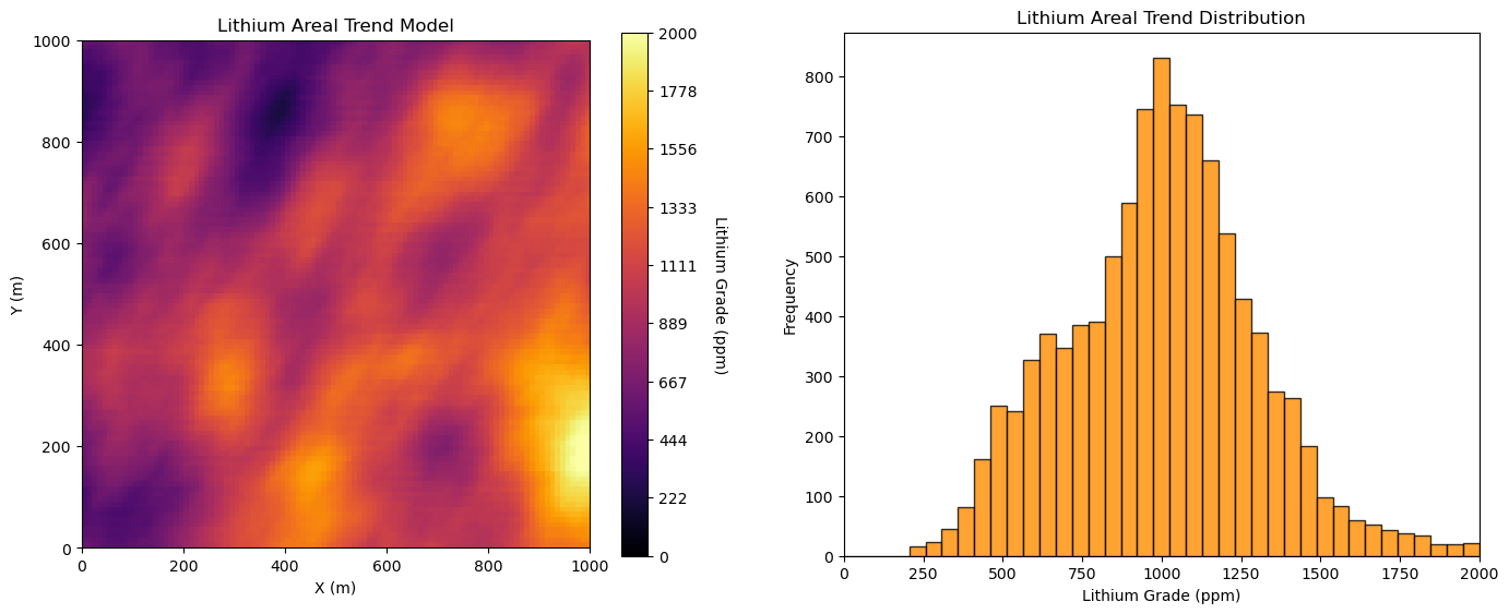
Load the 2D Areal Trend Model, \(\overline{Z}(\bf{𝐮}_{x},\bf{𝐮}_{y})\)#
We load the 2D trend model from my GeoDataSets repository.
lithium_areal_trend = np.loadtxt(r'https://raw.githubusercontent.com/GeostatsGuy/GeoDataSets/master/Lithium_Trend_Map.csv', delimiter=",")

global_mean = 1000.0
xmin=0; ymin=0; xmax=1000; ymax=1000;
vmin=0;vmax=2000

nx = 100; ny = 100; nz = 30
xsiz=10.0; ysiz=10.0; zsiz=1.0
xmn=xsiz/2; ymn=ysiz/2; zmn=zsiz/2

plt.subplot(121)
im = plt.imshow(lithium_areal_trend,interpolation = None,extent = [xmin,xmax,ymin,ymax], vmin = vmin, vmax = vmax,cmap = cmap)
plt.title('Lithium Areal Trend Model')
plt.xlabel('X (m)')
plt.ylabel('Y (m)')
cbar = plt.colorbar(im, orientation="vertical", ticks=np.linspace(vmin, vmax, 10))
cbar.set_label('Lithium Grade (ppm)', rotation=270, labelpad=20)

plt.subplot(122)
plt.hist(lithium_areal_trend.flatten(),bins=np.linspace(0,2000,40),color='darkorange',alpha=0.8,edgecolor='black')
plt.xlabel('Lithium Grade (ppm)'); plt.ylabel('Frequency'); plt.title('Lithium Areal Trend Distribution')
plt.xlim([0,2000])

plt.subplots_adjust(left=0.0, bottom=0.0, right=2.0, top=1.0, wspace=0.2, hspace=0.2); plt.show()
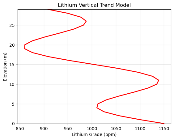
Assume a 1D Vertical Trend, \(\overline{Z}(\bf{𝐮}_{z})\)#
We assume a simple model with additive linear and periodic components.
vgradient = 10.0; amp = 100.0; lambd = 10

z = np.arange(0,30,1)
lithium_vertical_trend = (z-15)*-1*vgradient + amp*np.sin(3.1*lambd*z) + global_mean

plt.plot(lithium_vertical_trend,z,color='red',lw=2)
plt.ylim([0,29]); plt.grid()
plt.xlabel('Lithium Grade (ppm)'); plt.ylabel('Elevation (m)'); plt.title('Lithium Vertical Trend Model')
Text(0.5, 1.0, 'Lithium Vertical Trend Model')
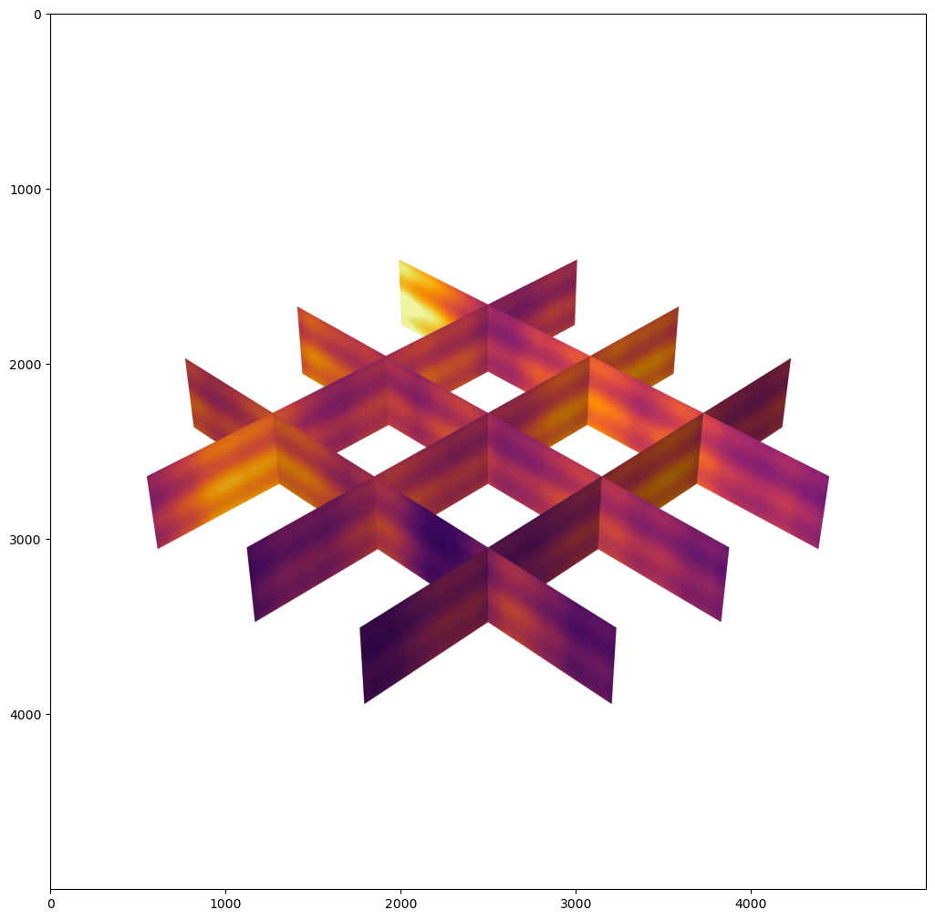
Calculate the 3D Trend, \(\overline{Z}(\bf{𝐮}_{x},\bf{𝐮}_{y},\bf{𝐮}_{z})\)#
Combine the 2D areal trend, 1D vertical trend and global mean to calculate the 3D trend model.
lithium_3D_trend = np.zeros([ny,nx,nz])

for iy in range(0,ny):
    for ix in range(0,nx):
        for iz in range(0,nz):
            lithium_3D_trend[iy,ix,iz] = lithium_vertical_trend[iz]*lithium_areal_trend[iy,ix]/global_mean
Visualize the 3D Trend Model#
Now let’s use PyVista to build a fence plot of the full 3D trend model.
xsections = [25,50,75]; ysections = [25,50,75]
zscalefactor = 0.5; opacity = 1.0

plt.subplot(111)
fence_diagram(lithium_3D_trend,xsections,ysections,zscalefactor);

plt.subplots_adjust(left=0.0, bottom=0.0, right=6.0, top=2.0, wspace=0.6, hspace=0.2); plt.show()
About the Author#

Michael Pyrcz is a professor in the Cockrell School of Engineering, and the Jackson School of Geosciences, at The University of Texas at Austin, where he researches and teaches subsurface, spatial data analytics, geostatistics, and machine learning. Michael is also,
the principal investigator of the Energy Analytics freshmen research initiative and a core faculty in the Machine Learn Laboratory in the College of Natural Sciences, The University of Texas at Austin
an associate editor for Computers and Geosciences, and a board member for Mathematical Geosciences, the International Association for Mathematical Geosciences.
Michael has written over 70 peer-reviewed publications, a Python package for spatial data analytics, co-authored a textbook on spatial data analytics, Geostatistical Reservoir Modeling and author of two recently released e-books, Applied Geostatistics in Python: a Hands-on Guide with GeostatsPy and Applied Machine Learning in Python: a Hands-on Guide with Code.
All of Michael’s university lectures are available on his YouTube Channel with links to 100s of Python interactive dashboards and well-documented workflows in over 40 repositories on his GitHub account, to support any interested students and working professionals with evergreen content. To find out more about Michael’s work and shared educational resources visit his Website.
Want to Work Together?#
I hope this content is helpful to those that want to learn more about subsurface modeling, data analytics and machine learning. Students and working professionals are welcome to participate.
Want to invite me to visit your company for training, mentoring, project review, workflow design and / or consulting? I’d be happy to drop by and work with you!
Interested in partnering, supporting my graduate student research or my Subsurface Data Analytics and Machine Learning consortium (co-PI is Professor John Foster)? My research combines data analytics, stochastic modeling and machine learning theory with practice to develop novel methods and workflows to add value. We are solving challenging subsurface problems!
I can be reached at mpyrcz@austin.utexas.edu.
I’m always happy to discuss,
Michael
Michael Pyrcz, Ph.D., P.Eng. Professor, Cockrell School of Engineering and The Jackson School of Geosciences, The University of Texas at Austin
More Resources Available at: Twitter | GitHub | Website | GoogleScholar | Geostatistics Book | YouTube | Applied Geostats in Python e-book | Applied Machine Learning in Python e-book | LinkedIn
Comments#
This was a basic demonstration of trend modeling to support 3D model construction. Much more can be done, I have other demonstrations for modeling workflows with GeostatsPy in the GitHub repository GeostatsPy_Demos.
I hope this is helpful,
Michael