

Convolutional Neural Networks#
Michael J. Pyrcz, Professor, The University of Texas at Austin
Twitter | GitHub | Website | GoogleScholar | Geostatistics Book | YouTube | Applied Geostats in Python e-book | Applied Machine Learning in Python e-book | LinkedIn
Chapter of e-book “Applied Machine Learning in Python: a Hands-on Guide with Code”.
Cite this e-Book as:
Pyrcz, M.J., 2024, Applied Machine Learning in Python: A Hands-on Guide with Code [e-book]. Zenodo. doi:10.5281/zenodo.15169139 ![]()
The workflows in this book and more are available here:
Cite the MachineLearningDemos GitHub Repository as:
Pyrcz, M.J., 2024, MachineLearningDemos: Python Machine Learning Demonstration Workflows Repository (0.0.3) [Software]. Zenodo. DOI: 10.5281/zenodo.13835312. GitHub repository: GeostatsGuy/MachineLearningDemos ![]()
By Michael J. Pyrcz
© Copyright 2024.
This chapter is a tutorial for / demonstration of Convolutional Neural Networks.
YouTube Lecture: check out my lectures on:
These lectures are all part of my Machine Learning Course on YouTube with linked well-documented Python workflows and interactive dashboards. My goal is to share accessible, actionable, and repeatable educational content. If you want to know about my motivation, check out Michael’s Story.
Motivation#
Convolutional neural networks are very powerful, nature inspired computing deep learning method based on an analogy of visual cortex extending the ability of our artificial neural networks to better work with images.
Nature inspired computing is looking to nature for inspiration to develop novel problem-solving methods,
artificial neural networks are inspired by biological neural networks
nodes in our model are artificial neurons, simple processors
connections between nodes are artificial synapses
perceptive fields regularization to improve generalization and efficiency
intelligence emerges from many connected simple processors. For the remainder of this chapter, I will used the terms nodes and connections to describe our convolutional neural network.
Concepts in Common with Artificial Neural Networks#
Here are some key aspects of artificial neural networks (ANNs),
Basic Design - “…a computing system made up of a number of simple, highly interconnected processing elements, which process information by their dynamic state response to external inputs.” Caudill (1989).
Still a Prediction Model - while these models may be quite complicated with even millions of trainable model parameters, weights and biases, they are still a function that maps from predictor features to response features,
Supervised learning – we provide training data with predictor features, \(X_1,\ldots,𝑋_𝑚\) and response feature(s), \(𝑌_1,\ldots,𝑌_K\), with the expectation of some model prediction error, \(\epsilon\).
Nonlinearity - nonlinearity is imparted to the system through the application of nonlinear activation functions to model nonlinear relationships
Universal Function Approximator (Universal Approximation Theorem) - artificial neural networks have the ability to learn any possible function shape of \(f\) over an interval, for an arbitrary wide (single hidden layer) by Cybenko (1989) and arbitrary depth by Lu and others (2017)
For brevity, I will not repeat all the fundamental concepts from the artificial neural network chapter.
it may be a good idea to review that chapter before starting with this one
Convolutional Neural Networks Concepts#
Regularization - artificial neural networks are prone to overfitting; therefore, we need a form of regularization to prevent this
for example, ridge and LASSO integrate regularization into the loss function through the shrinkage term to reduce overfit
With convolutional neural networks we take a different approach to regularization,
with image data we have an implicit hierarchy / proximity and relative position of pixels, flattening our 2D images into 1D vectors to pass through multiple fully connected artificial neural network layers would destroy this information
so we remove, regularize to 0.0, all connections outside of perceptive fields to preserve proximity and relative position of pixels information while avoiding overfit
these perceptive fields are regularization through extraction of smaller pixel subsets and simpler patterns from the images
Note, we also include dropout, random removal of connections, as another form of regularization
Image Data with Artificial Neural Networks#
We could use image data with our artificial neural networks.

What is the issue with this approach?
Massive number of model parameters - the model will likely be difficult to train and overfit.
Very sensitive to location - we would like to learn from our images with location invariance, i.e., for the example above the location of the channels should not matter.
Flattening the image to a vector - this is required by a artificial neural network, but if we first flatten our images to a vector we lose important information about the inter-pixel patterns, ordering, adjacency, etc.
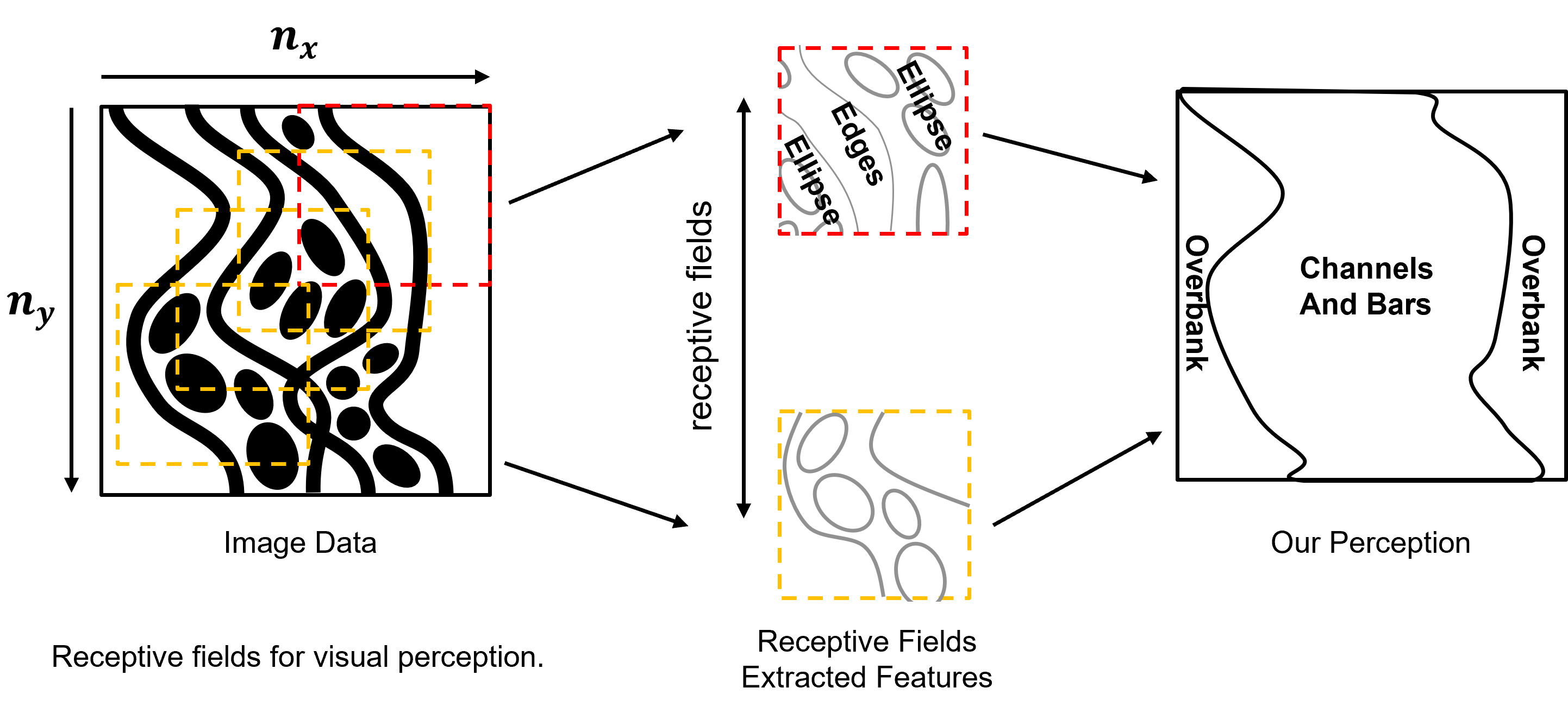
In summary, artificial neural networks are very inefficient for images and overfit and don’t generalize well! Instead, let’s be inspired by our visual cortex, with our vision we do not perceive all ‘pixels’, instead we segment the field of view into receptive fields.
we extraction of features of interest from overlapping receptive fields, over a hierarchy (not shown) and then recompose the whole image, our perception.
we don’t perceive all the ‘pixels’ that would be exhausting for our brains, instead our visual cortex interprets and summarizes patterns.
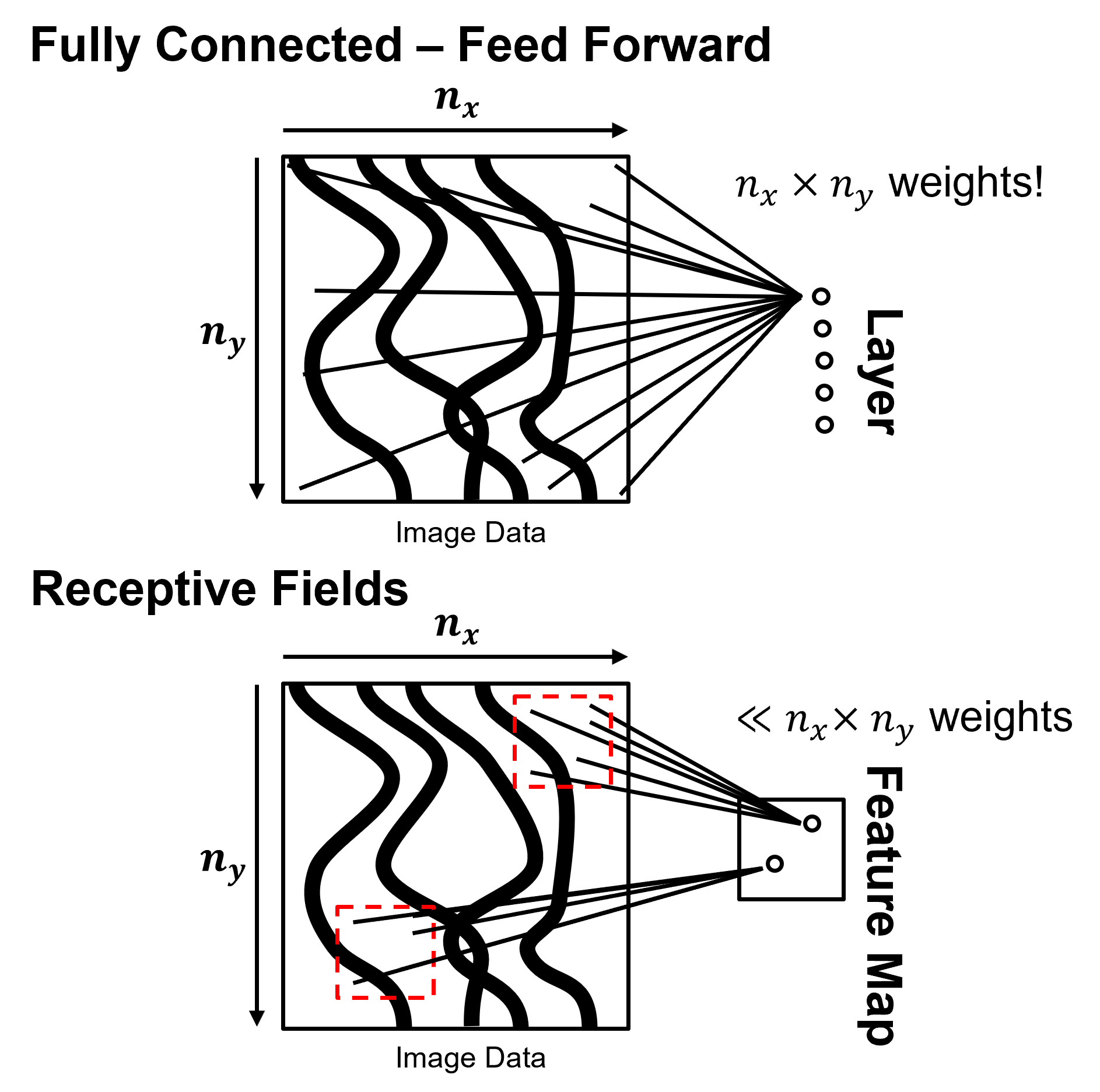
Now let’s compare artificial neural networks and convolutional neural networks with this concept of receptive fields.
Fully Connected, Feed Forward Artificial Neural Network
nodes in the next layer are connected to all nodes of the previous layer
spatial information is lost, the image data is immediately flattened to a 1D vector and adjacency / ordering information is lost
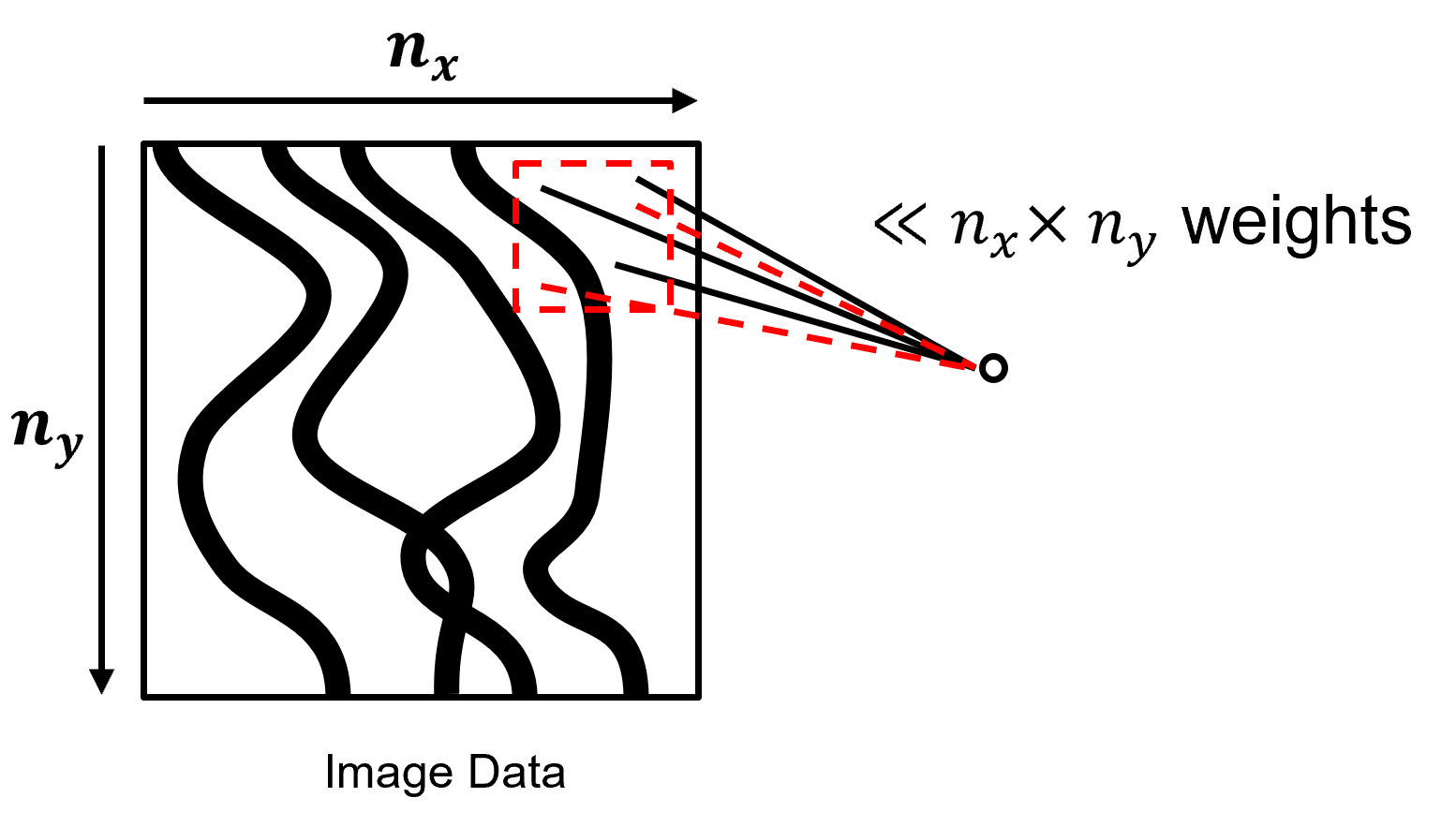
Regularized with Receptive Fields Convolutional Neural Networks
nodes in the next layer are mapped to specific regions of the previous layer, an image or feature map
spatial information is preserved, data retains the original image 2D or 3D dimensionality in each layer, called feature maps.
Regularization for CNNs#
Let’s do a quick recall on the concept of regularization for predictive machine learning models,
Regularization - a constraint to reduce the sensitivity of the model to the data, i.e., to reduce model variance
Regularization with Receptive Fields - the use of receptive fields is a form of regularization, resulting in,
massive reduction in connections, weights / model parameters
effectively shrinking these potential weights to zero
While integrating / focusing on pixel patterns!
Regularization with Dropout - during training epochs, randomly ignore or “drop out” a proportion of nodes. Each training epoch sees a different version / subset of the network
an additional form of regularization for CNN to prevent specific nodes from dominating the model
simulates training multiple models and averaging like ensemble learning. Note, it is generally not feasible to train multiple networks in parallel to apply the ensemble to calculate the prediction (like random forest) and after training all nodes are used.
Batch Normalization - standardize the nodes’ inputs / weights over a layer to center and rescale (mean of 0 and variance of 1) to optimize activation function sensitivity and model parameter training.
Then we add 2 model parameters, layer standard deviation, \(\gamma\), and mean, \(\beta\), to add control to improve the optimality of the train individual weights in the next layer.
Building Blocks for CNNs#
We have various operators to move from layer to layer (feature maps to feature maps) in our convolutional neural networks. The common operators include,
Convolution – a weighting window, kernel / filter designed to extract spatial information
Pooling – reduction in dimensionality, increase local translation invariance
Depth-wise Pooling, Down Sampling – 1x1 filter that combine channels / feature maps to learn over multiple kernels
Activation – use of an activation function to apply a nonlinear transformation to impart nonlinearity to the system and to prevent collapse of the system to a simple linear model
Full-connected, Feed Forward – see previous lecture on artificial neural networks
Now we will describe, interpret and demonstrate these operators.
Convolution#
Convolution is the integral product of two functions, after one is reversed and shifted by \(\Delta\).
one interpretation is smoothing a function with weighting function, \(𝑓(\Delta)\), is applied to calculate the weighted average of function, \(𝑔(x)\),
this easily extends into any dimensionality, for example 2D for images,
The choice of which function is shifted before integration does not change the result, the convolution operator has commutativity,
if either function is reflected then convolution is equivalent to cross-correlation, measure of similarity between 2 signals as a function of displacement.
To demonstrate convolution with an exhaustive \(g(x)\) and sparsely sampled \(g(x)\) I built out an interactive Python convolution dashboard,
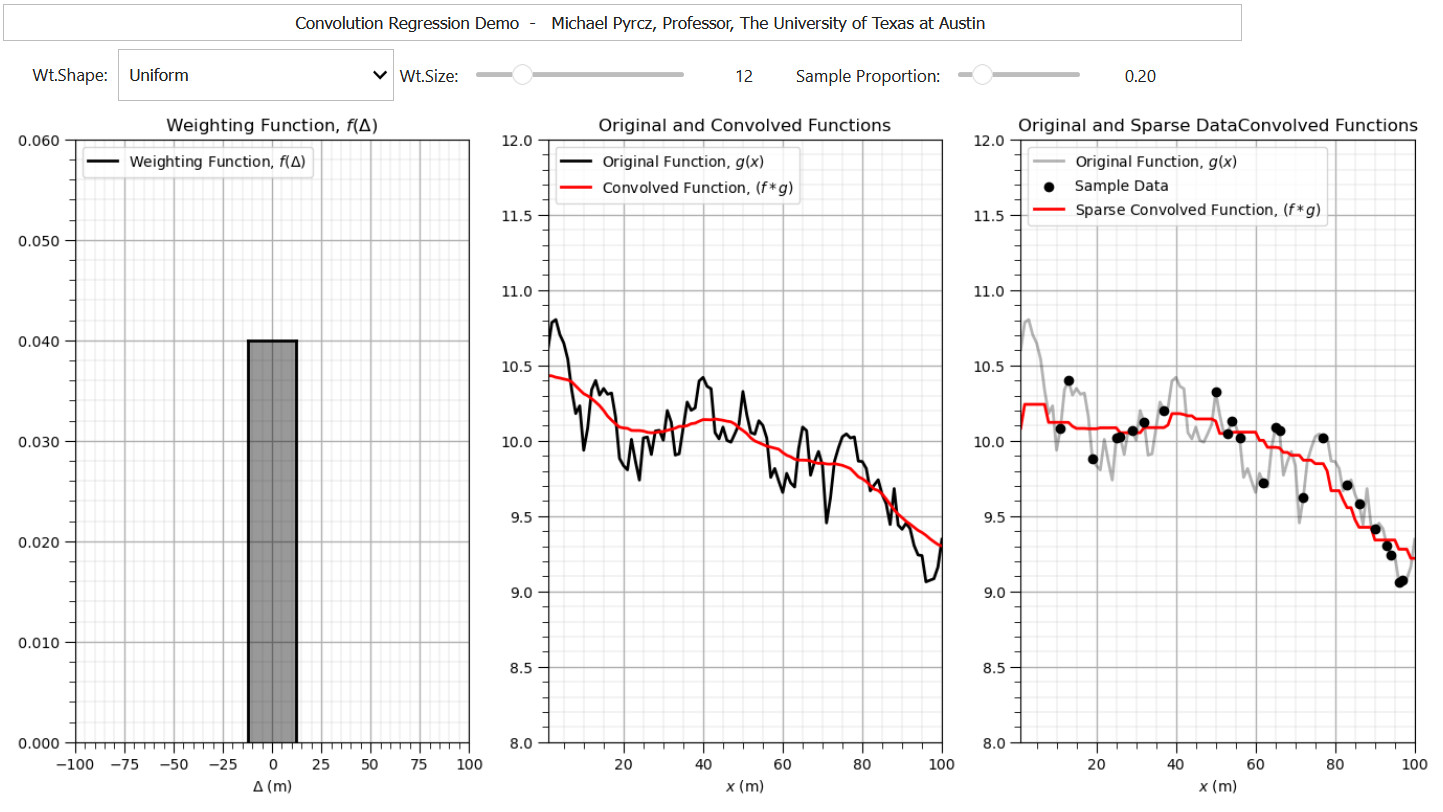
For convolution operations, a trainable weighting function, \(g(\Tau)\), is learned during model training.
Filter/Kernel – the weights assigned over the convolution window to calculate the next feature map. By training the weights the filter(s) may extract specific spatial features.
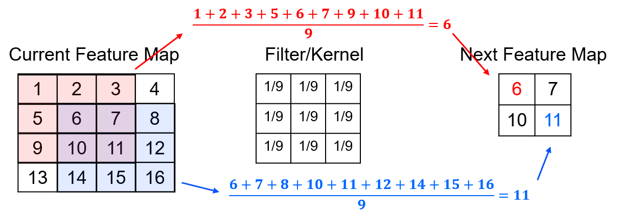
Let’s look at a specific kernel form, the blur filter.
the next feature map receives the local averages over the previous feature map or image.
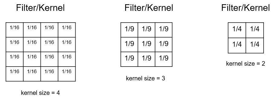
Some observations about the filters,
size of the filter is related to the scale of the features that we are extracting
larger kernels increase the number of connections, model weights and ultimately the computational complexity
odd numbers for kernel size to avoid distortion, asymmetric kernels are possible
sum to one prevent bias (shifting in the mean from one image or feature map to another feature map
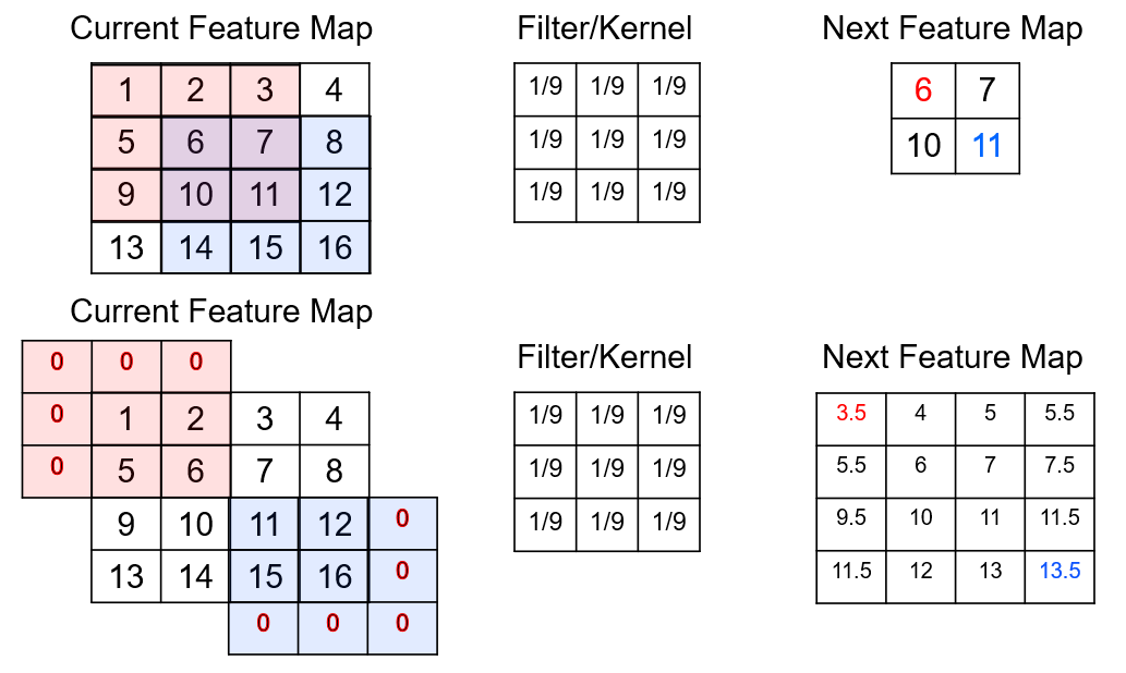
Padding - our next feature map has a reduced size by 1 on all the edges to avoid the overlapping outside the feature map, i.e., no padding, while padding extrapolates outside the feature map or image, preventing reduction in size of the next feature map.
there are varirous methods for padding, including assuming zero, constant value, and nearest value in feature map.
Stride - the steps of the convolution filter / kernel through the previous feature map.
for a stride of 1 there is no implicit reduction in feature map size.
for a stride of > 2 there is a reduction in feature map size.
Size of Next Feature Map - the next feature map size is determined by the hyperparameters, previous feature map size, \(n_{in}\), convolution kernel size, \(k\), convolution padding size, \(p\) and convolution stride size, \(s\), by this equation,
For example, if,
\(n_{in} = 4\)
\(k = 2\)
\(p = 0\)
\(s = 1\)
Then we can substitute into the equation,
Now compare this to a visualization of this example,
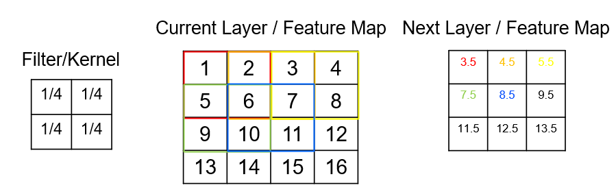
We calculate the next feature map size as:
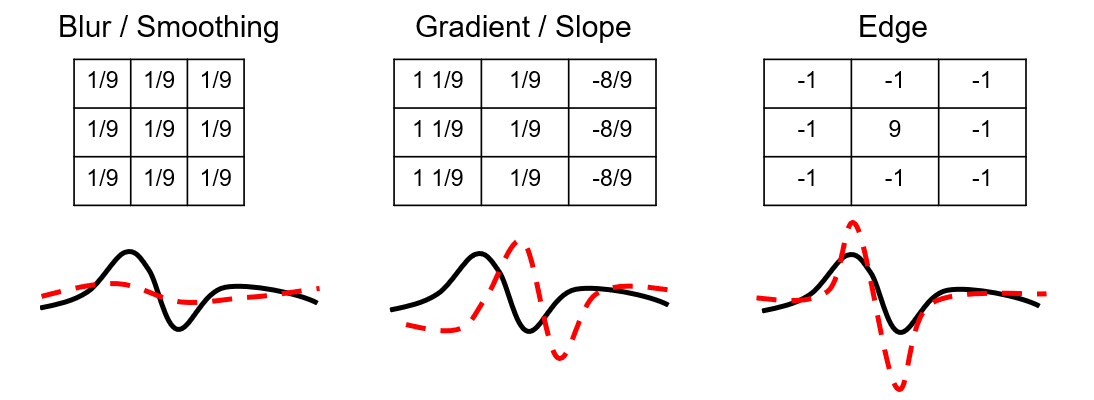
Filter / Kernel Design – by training the weights the filter may extract specific features. Consider these example filter types with simple 1D examples of input and output feature ‘maps’.
Multiple Filters / Kernels - typically multiple filters, \(n_k\), are trained on each convolutional layer to extract various structures from the image.
this increases feature map depth or channels, \(n_k\)
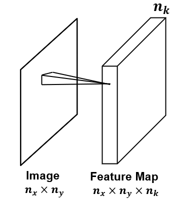
note, the original image may have multiple channels, depth > 1, for example, a RGB image with 3 channels, one for each red, blue and green.
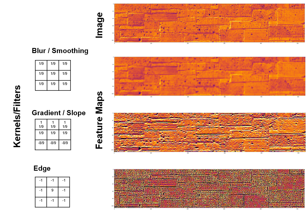
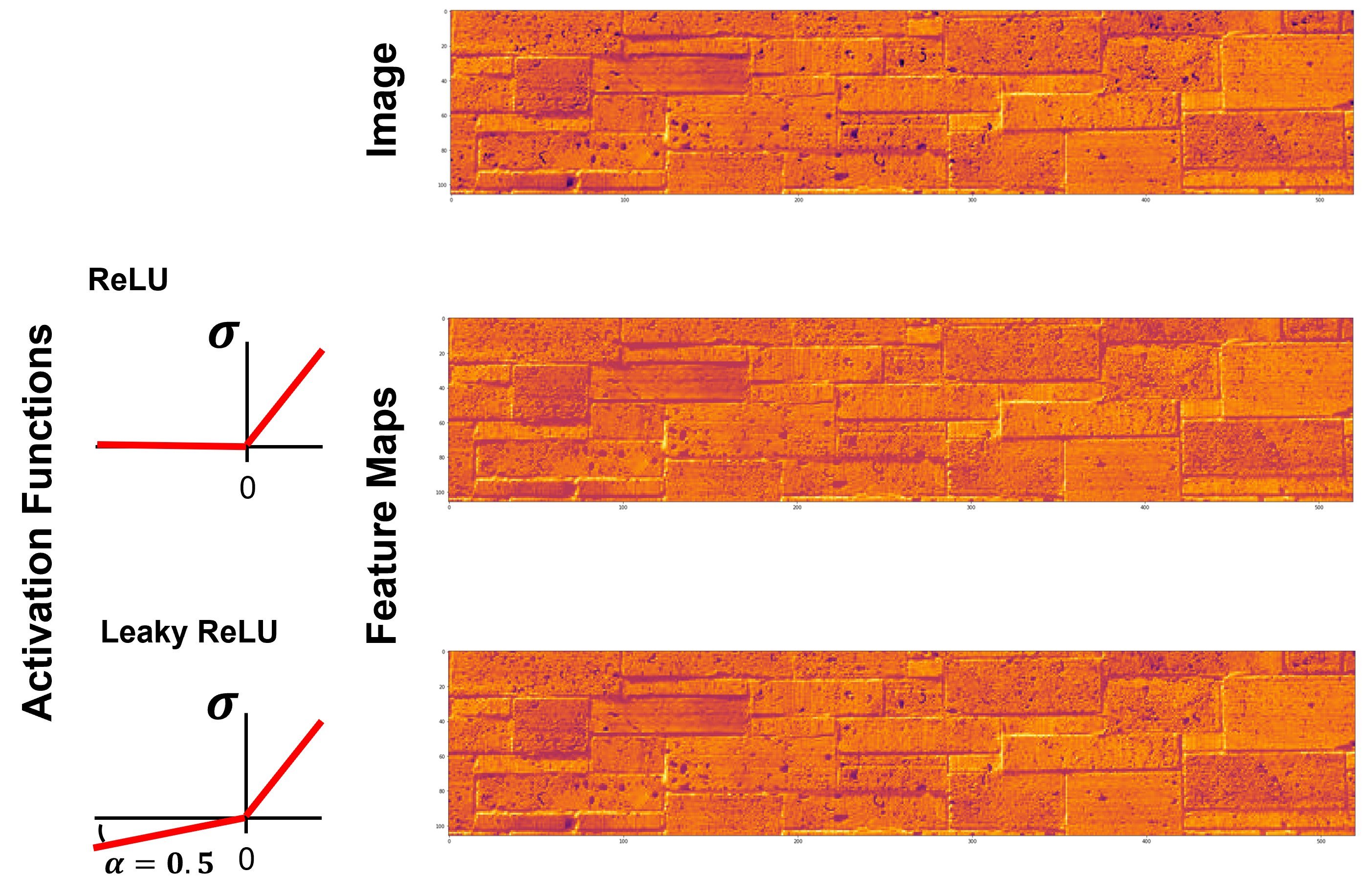
Finally here are some examples of convolution filters applied to an image of a brick wall on The University of Texas at Austin, codes are available at SubsurfaceDataAnalytics_Convolution_Operators.ipynb..
Activation Functions#
See the artificial neural network chapter for more details, but for a reminder considerations for selecting activation functions,
Nonlinear – required to impose nonlinearity into the predictor. Proved to be a universal function approximator if at least 1 hidden layer (Cybenko, 1989).
Range – finite for more stability gradient-based learning, infinite for more efficient training (but requires a slower learning rate)
Continuously Differentiable – required for stable gradient-based optimization
Smooth functions with Monotonic Derivative – may generalize better
Monotonic – guaranteed convexity of error surface of a single layer model (global minimum for loss function)
Approximates Identity at the Origin – well learn efficiently with the weights initialized with small random values
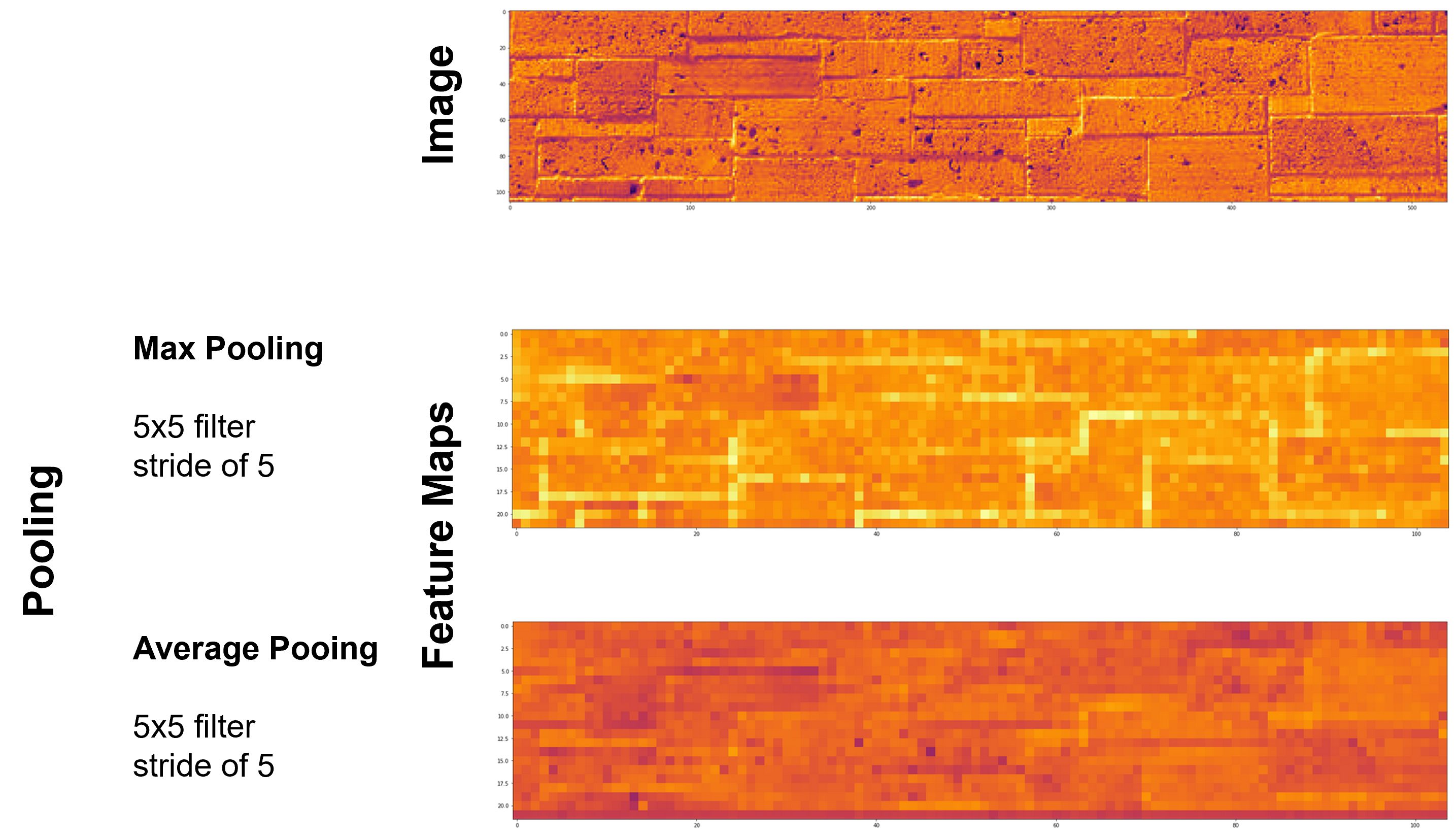
Pooling#
Summarization over a filter / kernel with a single value. The impact of pooling includes,
down sample the detection of features in feature maps
reduces the dimensionality of the feature map
integrate translation invariance, pattern detection insensitive to location
Two common pooling methods are average and max pooling.

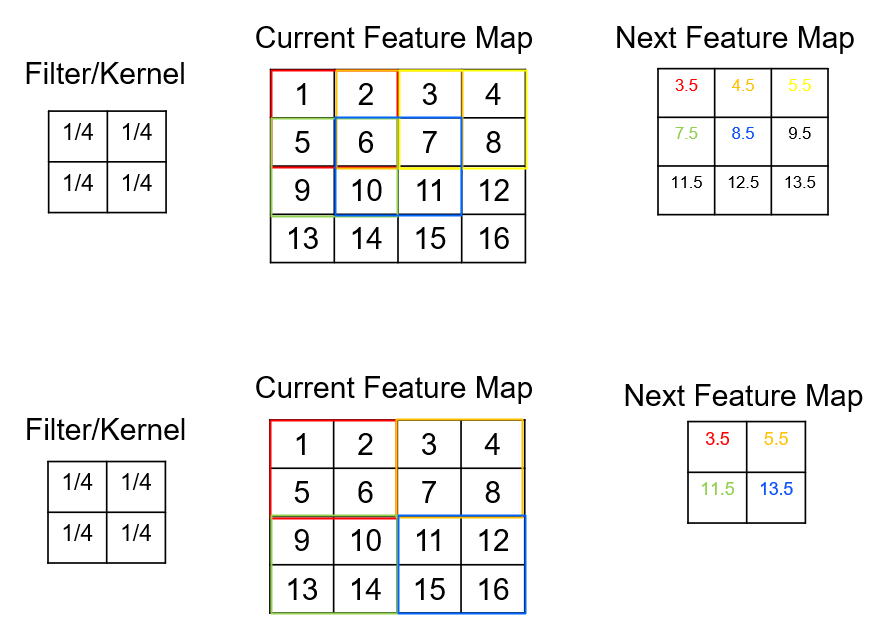
Here’s an example of pooling with a 2x2 filter and a stride of 2.
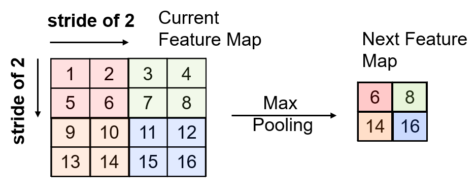
with 2 x 2 filter, stride of 2 the dimension is reduced ½ per axis, ¼ for 2D images.
for example, the value of 16 is location independent within the filter. This introduces translational invariance.
Depth-wise Pooling#
Summarization over feature maps with a single value.
down sample the detection over feature maps
combine information learned from multiple kernels
reduces the depth of the feature map, next layer
Two common pooling methods are average and max pooling.

Common CNN Architecture#
The following is a common workflow for convolutional neural networks,
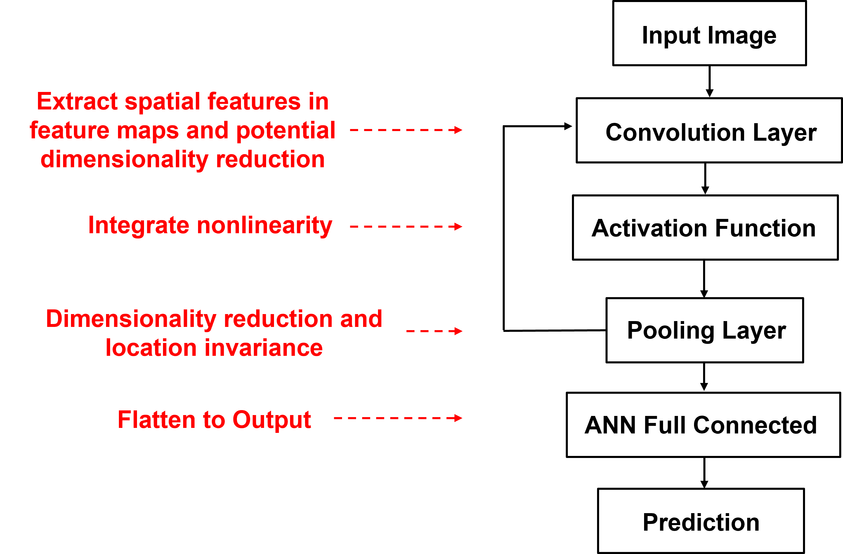
We can illustrate this common workflow with an illustration of the common architecture.

By-Hand CNN Architecture#
Just like the artificial neural network chapter, I build a simple convolutional neural network by-hand.
For simplicity and brevity, I have made the following architectural choices,
1D images with height of 5
1 convolutional layer with 1 kernel of size 3
activation with sigmoid
stride of 1 and no padding so the feature map has a size of 3
artificial neural network from feature map immediately to output node with linear activation
This minimalist architecture demonstrates many of the salient concepts for convolutional neural networks while being very easy to visualize and very fast to train.
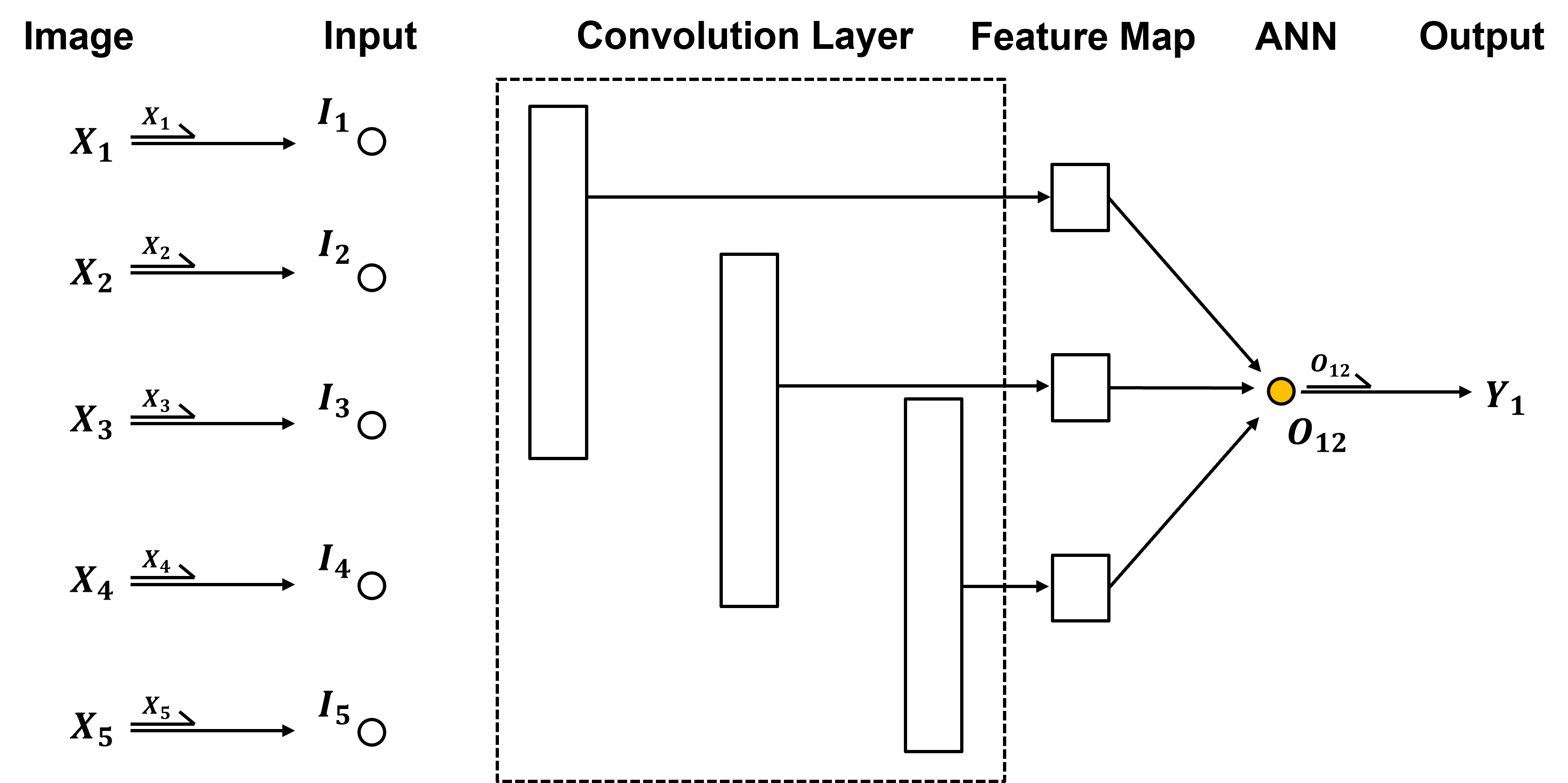
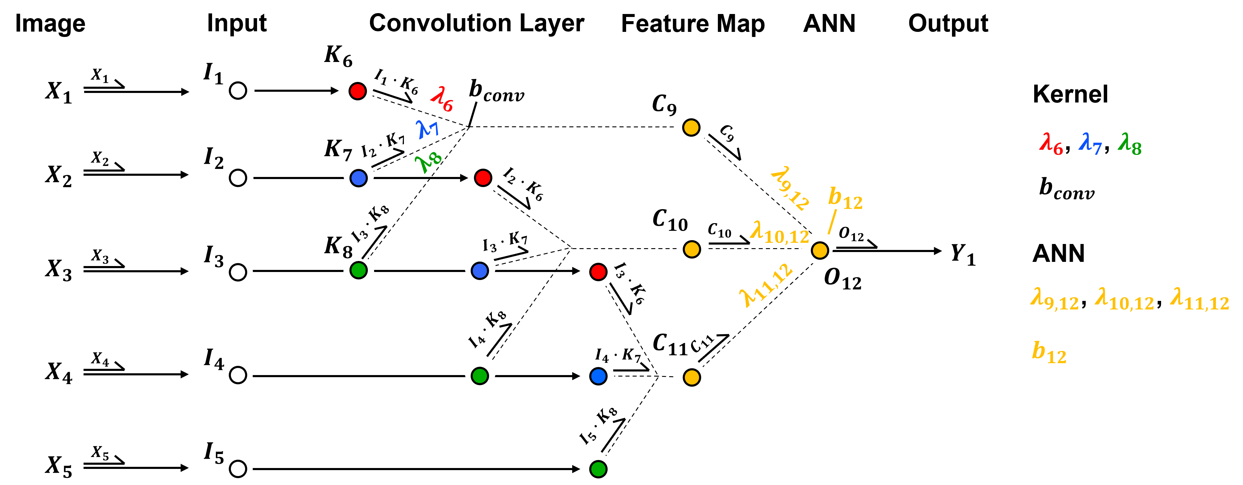
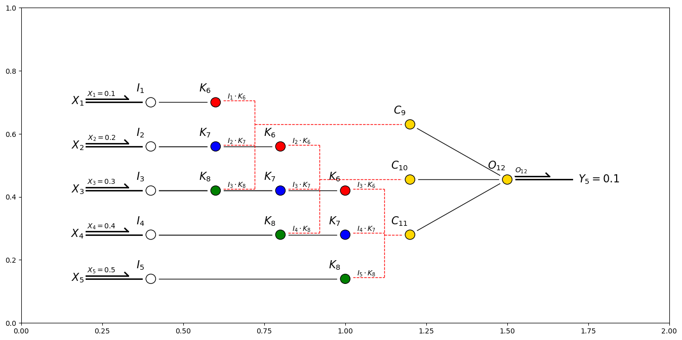
Now, we convert this schematic of our by-hand CNN to a diagram of the actual nodes.

To demonstrate the practicality of working with this architecture, let’s add the labels of the model parameters,
kernel weights, \(\lambda_6\), \(\lambda_7\), and \(\lambda_8\)
kernel bias, \(b_{conv}\)
artificial neural network weights, \(\lambda_{9,12}\), \(\lambda_{10,12}\), and \(\lambda_{11,12}\)
artificial neural network bias, \(b_{12}\)
Training Model Parameters#
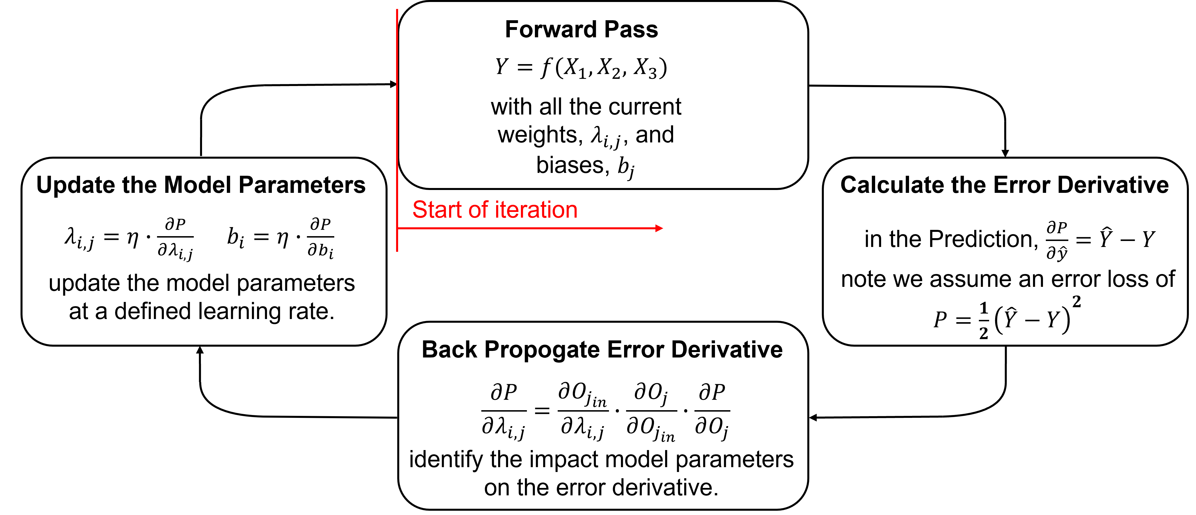
Training a convolutional neural network proceeds iteratively by these steps, the same as discussed in the artificial neural network chapter.
Here’s some details on each step with a focus on differences from artificial neural networks, for more details see the artificial neural network chapter.
Initializing the Model Parameters - initialize all model parameters with typically small (near zero) random values. Here’s a couple common methods,
Xavier Glorot Uniform Initialization - for Tanh and sigmoid activation, random realizations from uniform distributions specified by \(U[\text{min}, \text{max}]\),
where \(F^{-1}_U\) is the inverse of the CDF, \(p\) is the number of inputs, and \(p^{\ell}\) is a random cumulative probability value drawn from the uniform distribution, \(U[0,1]\).
For example, given a \(3 \times 3\) kernel with 1 channel in and 9 channel out,
He Kaiming Weight Initialization - for ReLU and leaky ReLU activation, random realizations from uniform distributions specified by \(U[\text{min}, \text{max}]\),
where \(F^{-1}_U\) is the inverse of the CDF, \(p\) is the number of inputs, \(k\) is the number of outputs, and \(p^{\ell}\) is a random cumulative probability value drawn from the uniform distribution, \(U[0,1]\).
Forward Pass - to make a prediction, \(\hat{y}\). Initial predictions will be random for the first iteration, but will improve.
Calculate the Error Derivative - given a loss of, \(P = \frac{1}{2} \left(\hat{y} - y \right)^2\), the error derivative, i.e., rate of change of in error given a change in model estimate is \(\frac{\partial P}{\partial \hat{y}} = \hat{Y} - Y\).
For now, let’s only consider a single estimate, and we will address more than 1 training data later.
Backpropagate the Error Derivative - we shift back through the artificial neural network to calculate the derivatives of the error over all the model weights and biases parameters, to accomplish this we use the chain rule,
Update the Model Parameters - based on the derivatives, \frac{\partial P}{\partial \lambda_{i,j}} and learning rates, \(\eta\), like this,
Repeat Until Convergence - return to step 1. until the error, \(P\), is reduced to an acceptable level, i.e., model convergence is the condition to stop the iterations
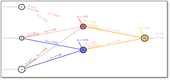
Backpropagation#
For brevity, I refer you to the artificial neural network chapter for a walkthrough of backpropagating the error gradient through a neural network.
Updating Model Parameters#
The derivatives for each of the model parameters are the error gradients, so we are ready to use gradient descent optimization with the addition of,
learning rate - to scale the rate of change of the model updates we assign a learning rate, \(\eta\). For our model parameter examples from above,
recall, this process of gradient calculation and model parameters, weights and biases, updating is iterated and is known as gradient descent optimization.
the goal is to explore the loss hypersurface, avoiding and escaping local minimums and ultimately finding the global minimum.
learning rate, also known as step size is commonly set between 0.0 and 1.0, note 0.01 is the default in Keras module of TensorFlow
Low Learning Rate – more stable, but a slower solution, may get stuck in a local minimum
High Learning Rate – may be unstable, but perhaps a faster solution, may diverge out of the global minimum
One strategy is to start with a high learning rate and then to decrease the learning rate over the iterations
Learning Rate Decay - set as > 0 to avoid mitigate oscillations,
Training Epochs#
This is a good time to talk about stochastic gradient descent optimization, first let’s define some common terms,
Batch Gradient Descent - updates the model parameters after passing through all of the data
Stochastic Gradient Descent - updates the model parameters over each sample data
Mini-batch Gradient Descent - updates the model parameter after passing through a single batch
With mini-batch gradient descent stochasticity is introduced through the use of subsets of the data, known as batches,
for example, if we divide our 100 samples into 4 batches, then we iterate over each batch separately
we speed up the individual updates, fewer data are faster to calculate, but we introduce more error
this often helps the training explore for the global minimum and avoid getting stuck in local minimums and along ridges in the loss hypersurface
Finally our last definition here,
epoch - is one pass over all of the data, so that would be 4 iterations of updating the model parameters if we have 4 mini-batches
There are many other considerations that I will add later including,
momentum
adaptive optimization
Now let’s build the above artificial neural network by-hand and visualize the solution!
this is by-hand so that you can see every calculation. I intentionally avoided using TensorFlow or PyTorch.
Training with Multiple Training Images#
The backpropagation is based on a single sample, i.e., training image and paired response feature value; therefore, to train over multiple images we must cycle over the,
forward pass
calculate error derivative
back propagate
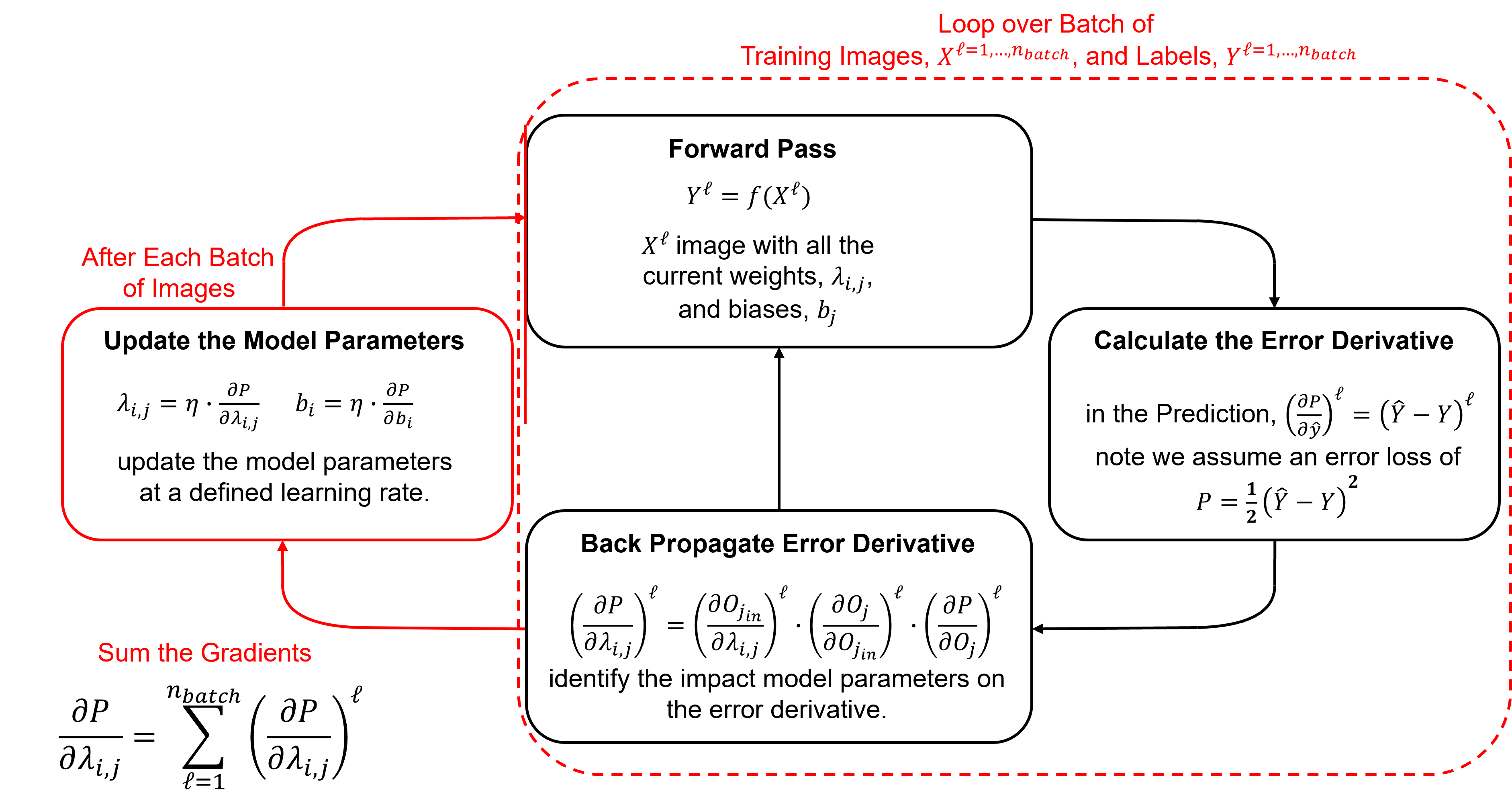
For each image the weights and biases gradients are stored. Then the gradients are summed over the images in the batch and this sum is applied with the learning rate to update the weights and biases.
Forward Pass#
For clarity, let’s walk through the convolutional neural network, starting with image input.
The input nodes receives the input from the image in to the convolution layer,
node order is retained to preserve spatial, location information from the image
For continuous feature images,
the continuous predictor feature values are normalized to a min / max of [0,1] or [-1,1] to improve sensitivity for the specific activation function
for color images, the RGB channels may be each normalized and included as 3 input channels
For categorical feature images,
for binary, cardinality of 2, the values may be reassigned by indicator transform to 0 or 1
for cardinality > 2, one-hot-encoding may be applied resulting in \(k\) input channels
See the feature transformation chapter for more details about these transformations.
Now we pass through a convolution layer, with convolution and activation, resulting in a new feature map.
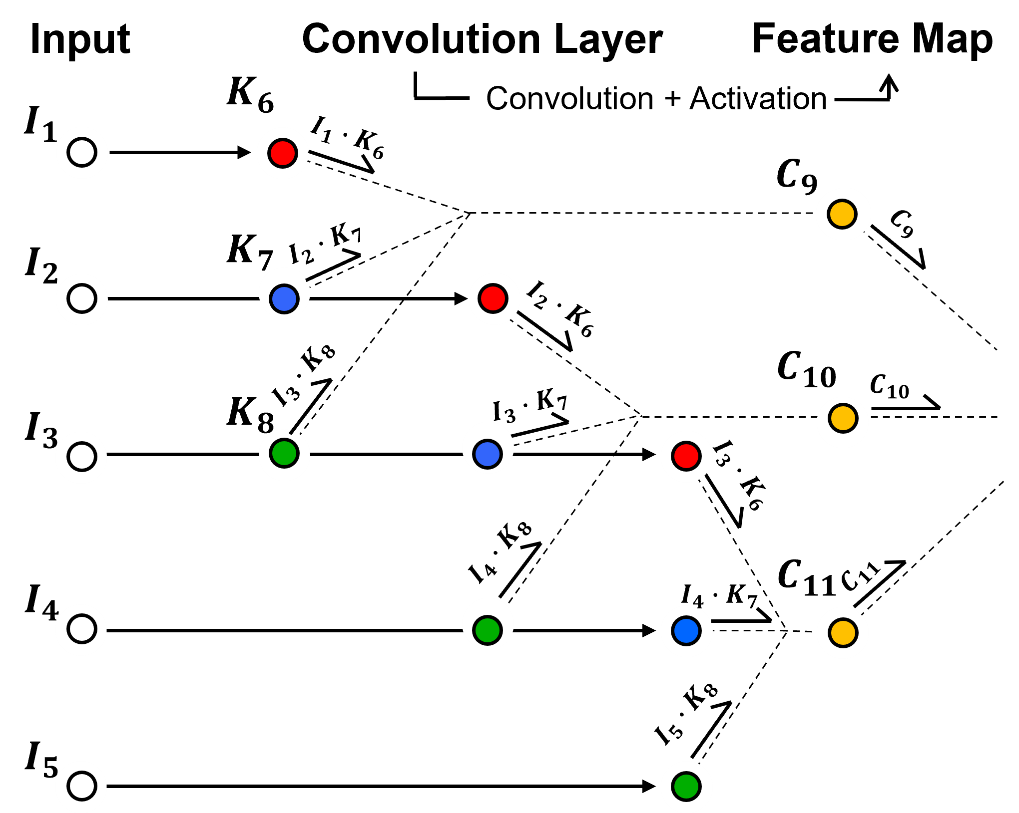
take linearly weighted combinations based on the kernel(s) of input image or previous feature map, add a bias term and then nonlinearly transform the result, this transform is call the activation function, \(\alpha\).
where, \(K_6\), \(K_7\) and \(K_8\) are kernel weights, \(b_{conv}\) is the kernel bias, and the \(I\) are the input nodes.
Please, excuse the strange indices in the equation, I like using unique node integers for every node to avoid mixing up nodes in my notes and codes, but this does complicate the index assignments.
then nonlinear activation is applied to each,
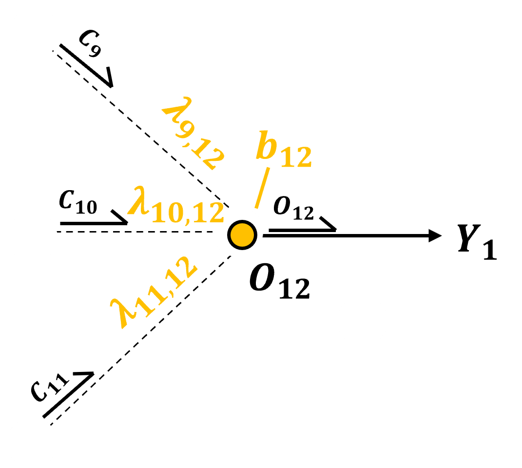
Now we proceed from the feature map through the artificial neural network to the output.
This is just a standard artificial neural network that takes the feature map flattened and moves it to the output.
in this example for brevity we show the simplest possible artificial neural network, i.e., the next layer after the feature map is the output. More complicated architectures with hidden layers are often applied.
also, since our images are 1D we do not require a flattening step
The output node is a standard output node from an artificial neural network,
input is a linear combination of the nodes from the previous layer with an added bias term.
and then an activation is applied,
For the case of a regression model, with continuous response feature, linear or identity activation is applied,
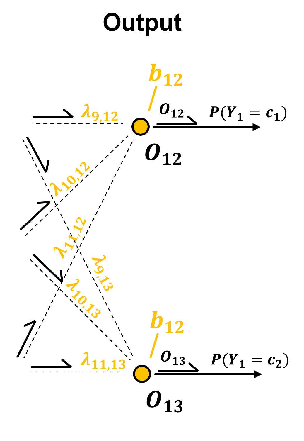
and for the case of a classification model, with categorical response feature, softmax activation is applied over \(K\) nodes equal to the cardinality of the response feature.
the output is a probability for each category that honors non-negativity and closure constraints
Import Required Packages#
We will also need some standard packages. These should have been installed with Anaconda 3.
recall our goal is to build a convolutional neural network by-hand with only basic math and array operations, so we only need NumPy along with matplotlib for plotting.
import numpy as np
import pandas as pd
import matplotlib.pyplot as plt
from matplotlib.ticker import (MultipleLocator, AutoMinorLocator, AutoLocator) # control of axes ticks
plt.rc('axes', axisbelow=True)                            # set axes and grids in the background for all plots
import math
seed = 13
If you get a package import error, you may have to first install some of these packages. This can usually be accomplished by opening up a command window on Windows and then typing ‘python -m pip install [package-name]’. More assistance is available with the respective package docs.
Declare Functions#
Here’s the functions to make, train and visualize our convoluational neural network.
def add_grid():
    plt.gca().grid(True, which='major',linewidth = 1.0); plt.gca().grid(True, which='minor',linewidth = 0.2) # add y grids
    plt.gca().tick_params(which='major',length=7); plt.gca().tick_params(which='minor', length=4)
    plt.gca().xaxis.set_minor_locator(AutoMinorLocator()); plt.gca().yaxis.set_minor_locator(AutoMinorLocator()) # turn on minor ticks

def calculate_angle_rads(x1, y1, x2, y2):
    dx = x2 - x1     # Calculate the differences
    dy = y2 - y1
    angle_rads = math.atan2(dy, dx)    # Calculate the angle in radians
    #angle_degrees = math.degrees(angle_radians)    # Convert the angle to degrees
    return angle_rads

def offset(pto, distance, angle_deg): # modified from ChatGPT 4.o generated
    angle_rads = math.radians(angle_deg) # Convert angle from degrees to radians
    x_new = pto[0] + distance * math.cos(angle_rads) # Calculate the new coordinates
    y_new = pto[1] + distance * math.sin(angle_rads)
    return np.array((x_new, y_new))

def offsetx(xo, distance, angle_deg): # modified from ChatGPT 4.o generated
    angle_rads = math.radians(angle_deg) # Convert angle from degrees to radians
    x_new = xo + distance * math.cos(angle_rads) # Calculate the new coordinates
    return np.array((xo, x_new))

def offset_arrx(xo, distance, angle_deg,size): # modified from ChatGPT 4.o generated
    angle_rads = math.radians(angle_deg) # Convert angle from degrees to radians
    x_new = xo + distance * math.cos(angle_rads) # Calculate the new coordinates
    x_arr = x_new + size * math.cos(angle_rads+2.48) # Calculate the new coordinates
    return np.array((x_new, x_arr))

def offsety(yo, distance, angle_deg): # modified from ChatGPT 4.o generated
    angle_rads = math.radians(angle_deg) # Convert angle from degrees to radians
    y_new = yo + distance * math.sin(angle_rads) # Calculate the new coordinates
    return np.array((yo, y_new))

def offset_arry(yo, distance, angle_deg,size): # modified from ChatGPT 4.o generated
    angle_rads = math.radians(angle_deg) # Convert angle from degrees to radians
    y_new = yo + distance * math.sin(angle_rads) # Calculate the new coordinates
    y_arr = y_new + size * math.sin(angle_rads+2.48) # Calculate the new coordinates
    return np.array((y_new, y_arr))

def lint(x1, y1, x2, y2, t):
    # Calculate the interpolated coordinates
    x = x1 + t * (x2 - x1)
    y = y1 + t * (y2 - y1)
    return np.array((x, y))

def lintx(x1, y1, x2, y2, t):
    # Calculate the interpolated coordinates
    x = x1 + t * (x2 - x1)
    return x

def linty(x1, y1, x2, y2, t):
    # Calculate the interpolated coordinates
    y = y1 + t * (y2 - y1)
    return y

def lint_intx(x1, y1, x2, y2, ts, te):
    # Calculate the interpolated coordinates
    xs = x1 + ts * (x2 - x1)
    xe = x1 + te * (x2 - x1)
    return np.array((xs,xe))

def lint_inty(x1, y1, x2, y2, ts, te):
    # Calculate the interpolated coordinates
    ys = y1 + ts * (y2 - y1)
    ye = y1 + te * (y2 - y1)
    return np.array((ys,ye))

def lint_int_arrx(x1, y1, x2, y2, ts, te, size):
    # Calculate the interpolated coordinates
    xe = x1 + te * (x2 - x1)
    line_angle_rads = calculate_angle_rads(x1, y1, x2, y2)
    x_arr = xe + size * math.cos(line_angle_rads+2.48) # Calculate the new coordinates
    return np.array((xe,x_arr))

def lint_int_arry(x1, y1, x2, y2, ts, te, size):
    # Calculate the interpolated coordinates
    ye = y1 + te * (y2 - y1)
    line_angle_rads = calculate_angle_rads(x1, y1, x2, y2)
    y_arr = ye + size * math.sin(line_angle_rads+2.48) # Calculate the new coordinates
    return np.array((ye,y_arr))

def as_si(x, ndp): # from xnx on StackOverflow https://stackoverflow.com/questions/31453422/displaying-numbers-with-x-instead-of-e-scientific-notation-in-matplotlib
    s = '{x:0.{ndp:d}e}'.format(x=x, ndp=ndp)
    m, e = s.split('e')
    return r'{m:s}\times 10^{{{e:d}}}'.format(m=m, e=int(e))
The Simple By-hand CNN#
I wrote this code to specify a simple CNN,
five input nodes, 1 convolution layer with a kernel of 3 resulting in a 3 nodes in the feature map and 1 output node
and to train the CNN by iteratively performing the forward calculation and backpropagation. I calculate:
the error and then propagate it to each node
solve for the partial derivatives of the error with respect to each weight and bias
all weights, biases and partial derivatives for all epoch are recorded in vectors for plotting
# initial CNN trains on one sample
x1 = 0.1; x2 = 0.2; x3 = 0.3; x4 = 0.4; x5 = 0.5; y = 0.1 # training data
lr = 0.2 # learning rate

np.random.seed(seed=seed)

nepoch = 1000

w6 = np.zeros(nepoch); w7 = np.zeros(nepoch); w8 = np.zeros(nepoch)
w9 = np.zeros(nepoch); w10 = np.zeros(nepoch); w11 = np.zeros(nepoch)
bconv = np.zeros(nepoch); b12 = np.zeros(nepoch)

k6i1 = np.zeros(nepoch); k6i2 = np.zeros(nepoch); k6i3 = np.zeros(nepoch)
k7i2 = np.zeros(nepoch); k7i3 = np.zeros(nepoch); k7i4 = np.zeros(nepoch)
k8i3 = np.zeros(nepoch); k8i4 = np.zeros(nepoch); k8i5 = np.zeros(nepoch)

dk6i1 = np.zeros(nepoch); dk6i2 = np.zeros(nepoch); dk6i3 = np.zeros(nepoch)
dk7i2 = np.zeros(nepoch); dk7i3 = np.zeros(nepoch); dk7i4 = np.zeros(nepoch)
dk8i3 = np.zeros(nepoch); dk8i4 = np.zeros(nepoch); dk8i5 = np.zeros(nepoch)

c9 = np.zeros(nepoch); c10 = np.zeros(nepoch); c11 = np.zeros(nepoch)
d9 = np.zeros(nepoch); d10 = np.zeros(nepoch); d11 = np.zeros(nepoch)

o12 = np.zeros(nepoch)

dw6 = np.zeros(nepoch); dw7 = np.zeros(nepoch); dw8 = np.zeros(nepoch)
dw9 = np.zeros(nepoch); dw10 = np.zeros(nepoch); dw11 = np.zeros(nepoch)
dbconv = np.zeros(nepoch); db12 = np.zeros(nepoch)

d6 = np.zeros(nepoch); d7 = np.zeros(nepoch); d8 = np.zeros(nepoch);
d19 = np.zeros(nepoch); d10 = np.zeros(nepoch); d11 = np.zeros(nepoch); d12 = np.zeros(nepoch);

# initialize the weights - Xavier Weight Initialization
lower, upper = -(1.0 / np.sqrt(3.0)), (1.0 / np.sqrt(3.0)) # lower and upper bound for the weights, uses inputs to node
#lower, upper = -(sqrt(6.0) / sqrt(3.0 + 2.0)), (sqrt(6.0) / sqrt(3.0 + 2.0)) # Normalized Xavier weights, integrates ouputs also
w6[0] = lower + np.random.random() * (upper - lower);
w7[0] = lower + np.random.random() * (upper - lower);
w8[0] = lower + np.random.random() * (upper - lower);

lower, upper = -(1.0 / np.sqrt(2.0)), (1.0 / np.sqrt(2.0))
#lower, upper = -(sqrt(6.0) / sqrt(2.0 + 1.0)), (sqrt(6.0) / sqrt(2.0 + 1.0)) # Normalized Xavier weights, integrates ouputs also

w9[0] = lower + np.random.random() * (upper - lower);
w10[0] = lower + np.random.random() * (upper - lower);
w11[0] = lower + np.random.random() * (upper - lower);

#b4[0] = np.random.random(); b5[0] = np.random.random(); b6[0] = np.random.random()
bconv[0] = (np.random.random()-0.5)*0.5
b12[0] = (np.random.random()-0.5)*0.5; # small random value

for i in range(0,nepoch):

# forward pass of model
    c9[i] = w6[i]*x1 + w7[i]*x2 + w8[i]*x3 + bconv[i];
    c9[i] = 1.0/(1 + math.exp(-1*c9[i]))

    c10[i] = w6[i]*x2 + w7[i]*x3 + w8[i]*x4 + bconv[i];
    c10[i] = 1.0/(1 + math.exp(-1*c10[i]))

    c11[i] = w6[i]*x3 + w7[i]*x4 + w8[i]*x5 + bconv[i];
    c11[i] = 1.0/(1 + math.exp(-1*c11[i]))

    o12[i] = w9[i]*c9[i] + w10[i]*c10[i] + w11[i]*c11[i] + b12[i]

# back propagate the error through the nodes
    d12[i] = (o12[i]-y) # identity activation o at o12 - switched substraction on May 27, 2025
    d9[i] =  c9[i]*(1-c9[i])*w9[i]*d12[i]   # propagate to the front feature map layer
    d10[i] = c10[i]*(1-c10[i])*w10[i]*d12[i]
    d11[i] = c11[i]*(1-c11[i])*w11[i]*d12[i]

    dk6i1 = x1*d9[i]; dk7i2 = x2*d9[i]; dk8i3 = x3*d9[i]
    dk6i2 = x2*d10[i]; dk7i3 = x3*d10[i]; dk8i4 = x4*d10[i]
    dk6i3 = x3*d11[i]; dk7i4 = x4*d11[i]; dk8i5 = x5*d11[i]

    d6[i] = dk6i1 + dk6i2 + dk6i3
    d7[i] = dk7i2 + dk7i3 + dk7i4
    d8[i] = dk8i3 + dk8i4 + dk8i5

# calculate the change in weights
    if i < nepoch - 1:
        dw6[i] = lr*d6[i]; dw7[i] = lr*d7[i]; dw8[i] = lr*d8[i]
        dw9[i] = lr*c9[i]*d12[i]; dw10[i] = lr*c10[i]*d12[i]; dw11[i] = lr*c11[i]*d12[i];
        dbconv[i] = lr*(d9[i] + d10[i] + d11[i]); db12[i] = lr*d12[i]

        w6[i+1] = w6[i] - dw6[i]; w7[i+1] = w7[i] - dw7[i]; w8[i+1] = w8[i] - dw8[i]
        w9[i+1] = w9[i] - dw9[i]; w10[i+1] = w10[i] - dw10[i]; w11[i+1] = w11[i] - dw11[i]
        bconv[i+1] = bconv[i] - dbconv[i]; b12[i+1] = b12[i] - db12[i]
Visualize By-hand CNN#
Let’s visualize our convolutional neural network.
note, I will used this code latter to make interactive dashboards.
xin = 0.1; yin_range = 0.7
nin = 5

kcolors = ['red','blue','green']
xin = np.array([0.1,0.2,0.3,0.4,0.5])
yout = np.array([y])
cin = np.array([0.1,0.2,0.3])
kx = 0.6

plt.subplot(111)
#plt.gca().set_axis_off()

for i, (xi) in enumerate(zip(xin), start=1):
    eq1 = r"$X_{{{}}}$".format(i)
    eq2 = r"$X_{{{}}} = {}$".format(i, xi[0])
    eq3 = r"$I_{{{}}}$".format(i)
    xpos = 0.4; ypos = yin_range - ((i-1)/nin) * yin_range
    circle_i1 = plt.Circle((xpos,ypos), 0.015, fill=False, edgecolor = 'black',lw=1,zorder=100);
    circle_i1b = plt.Circle((xpos,ypos), 0.025, fill=True, facecolor = 'white',edgecolor = None,lw=0.5,zorder=10);
    plt.gca().add_patch(circle_i1); plt.gca().add_patch(circle_i1b)
    plt.annotate(eq1, (xpos-0.2, ypos), textcoords="offset points", xytext=(-12, -3), ha='center',size=15)
    plt.annotate(eq2, (xpos, ypos), textcoords="offset points", xytext=(-70, 9), ha='center')
    plt.plot([xpos-0.2,xpos],[ypos,ypos],color='black',lw=2); plt.plot([xpos-0.2,xpos-0.07],[ypos+0.01,ypos+0.01],color='black',lw=2)
    plt.plot([xpos-0.07,xpos-0.08],[ypos+0.01,ypos+0.02],color='black',lw=2)
    plt.annotate(eq3, (xpos,ypos), textcoords="offset points", xytext=(-15, 15), ha='center',size = 15)

for iconv in range(0,3):
    xpos = kx+iconv*0.2;
    ytop = yin_range - (iconv/nin)*yin_range - ((1-1)/nin) * yin_range
    ybot = yin_range - (iconv/nin)*yin_range - ((3-1)/nin) * yin_range
    plt.plot([xpos+0.12,xpos+0.12],[ytop+0.005,ybot+0.005],color='red',lw=1,ls='--',zorder=80)
    for ik, (ki) in enumerate(zip(np.arange(1,4,1)), start=1):
        eq4 = r"$K_{{{}}}$".format(ik+5)
        ypos = yin_range - (iconv/nin)*yin_range - ((ik-1)/nin) * yin_range
        circle_i1 = plt.Circle((xpos,ypos), 0.015, fill=True, facecolor = kcolors[ik-1],edgecolor = 'black',lw=1,zorder=200);
        circle_i1b = plt.Circle((xpos,ypos), 0.025, fill=True, facecolor='white',edgecolor = None,lw=0.5,zorder=190);
        plt.gca().add_patch(circle_i1); plt.gca().add_patch(circle_i1b)
        plt.annotate(eq4, (xpos,ypos), textcoords="offset points", xytext=(-15, 15), ha='center',size = 15)
        plt.plot([0.4,xpos],[ypos,ypos],color='black',lw=1,zorder=1)
        plt.plot([xpos,xpos+0.12],[ypos+0.005,ypos+0.005],color='red',lw=1,ls='--',zorder=80)
        eq8 = r"$I_{{{}}} \cdot K_{{{}}}$".format((iconv)+ik,ik+5)
        plt.annotate(eq8, (xpos+0.12, ypos), textcoords="offset points", xytext=(-25, 5), ha='center',size = 10)

for ic, (ci) in enumerate(zip(np.arange(1,4,1)), start=1):
    eq5 = r"$C_{{{}}}$".format(ic+8)
    xpos = 1.2; ypos = yin_range - ((ic-1)/4) * yin_range - 0.07
    circle_i1 = plt.Circle((xpos,ypos), 0.015, fill=True, facecolor = 'gold',edgecolor = 'black',lw=1,zorder=200);
    circle_i1b = plt.Circle((xpos,ypos), 0.025, fill=True, facecolor='white',edgecolor = None,lw=0.5,zorder=190);
    plt.gca().add_patch(circle_i1); plt.gca().add_patch(circle_i1b)
    plt.annotate(eq5, (xpos,ypos), textcoords="offset points", xytext=(-15, 15), ha='center',size = 15)
    #plt.plot([0.4,x],[y,y],color='black',lw=1,zorder=1)
    plt.plot([xpos,1.5],[ypos,yin_range - ((2-1)/4) * yin_range - 0.07],color='black',lw=1)
    plt.plot([kx+(ic-1)*0.2+0.12,xpos],[ypos,ypos],color='red',lw=1,ls='--',zorder=80)


eq6 = r"$O_{{{}}}$".format(12)
eq7 = r"$Y_{{{}}} = {}$".format(i, np.round(yout[0],2))
xpos = 1.5; ypos = yin_range - ((2-1)/4) * yin_range - 0.07
circle_i1 = plt.Circle((xpos,ypos), 0.015, fill=True, facecolor = 'gold',edgecolor = 'black',lw=1,zorder=200);
circle_i1b = plt.Circle((xpos,ypos), 0.025, fill=True, facecolor='white',edgecolor = None,lw=0.5,zorder=190);
plt.gca().add_patch(circle_i1); plt.gca().add_patch(circle_i1b)
plt.annotate(eq6, (xpos, ypos), textcoords="offset points", xytext=(-15, 15), ha='center',size = 15)
plt.annotate(eq7, (xpos, ypos), textcoords="offset points", xytext=(130,-4), ha='center',size = 15)
plt.plot([xpos,xpos+0.2],[ypos,ypos],color='black',lw=2); plt.plot([xpos,xpos+0.13],[ypos+0.01,ypos+0.01],color='black',lw=2)
plt.plot([xpos+0.13,xpos+0.12],[ypos+0.01,ypos+0.02],color='black',lw=2)
plt.annotate(eq6, (xpos, ypos), textcoords="offset points", xytext=(20, 10), ha='center')


plt.xlim([0.,2.]); plt.ylim([0,1])

plt.subplots_adjust(left=0.0, bottom=0.0, right=2.0, top=1.3, wspace=0.2, hspace=0.2); plt.show()
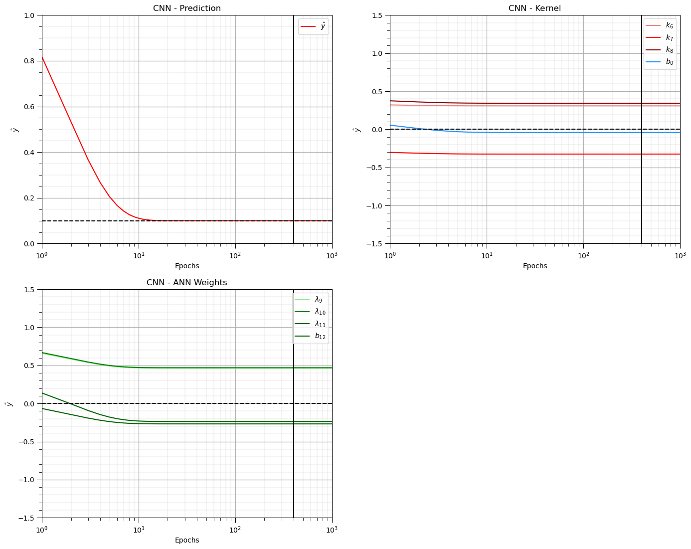
and now we can visualize the model training results including,
weights and biases vs. training epochs
CNN prediction vs. training epochs
plt.subplot(221)
plt.plot(np.arange(1,nepoch+1,1),o12,color='red',label=r'$\hat{y}$'); plt.xlim([1,nepoch]); plt.ylim([0,1])
plt.xlabel('Epochs'); plt.ylabel(r'$\hat{y}$'); plt.title('CNN - Prediction')
plt.plot([1,nepoch],[y,y],color='black',ls='--'); plt.vlines(400,-1.5,1.5,color='black')
add_grid(); plt.legend(loc='upper right'); plt.xscale('log')

plt.subplot(222)
plt.plot(np.arange(1,nepoch+1,1),w6,color='lightcoral',label = r'$k_6$')
plt.plot(np.arange(1,nepoch+1,1),w7,color='red',label = r'$k_7$')
plt.plot(np.arange(1,nepoch+1,1),w8,color='darkred',label = r'$k_8$')
plt.plot(np.arange(1,nepoch+1,1),bconv,color='dodgerblue',label = r'$b_0$')
# plt.plot(np.arange(1,nepoch+1,1),w25,color='blue',label = r'$\lambda_{2,5}$')
# plt.plot(np.arange(1,nepoch+1,1),w35,color='darkblue',label = r'$\lambda_{3,5}$')
# plt.plot(np.arange(1,nepoch+1,1),w46,color='orange',label = r'$\lambda_{4,6}$')
# plt.plot(np.arange(1,nepoch+1,1),w56,color='darkorange',label = r'$\lambda_{5,6}$')
plt.plot([1,nepoch],[0,0],color='black',ls='--')
plt.xlim([1,nepoch]); plt.ylim([-1.5,1.5]); plt.vlines(400,-1.5,1.5,color='black')
plt.xlabel('Epochs'); plt.ylabel(r'$\hat{y}$'); plt.title('CNN - Kernel')
add_grid(); plt.legend(loc='upper right'); plt.xscale('log')

plt.subplot(223)
plt.plot(np.arange(1,nepoch+1,1),w9,color='lightgreen',label = r'$\lambda_{9}$')
plt.plot(np.arange(1,nepoch+1,1),w10,color='green',label = r'$\lambda_{10}$')
plt.plot(np.arange(1,nepoch+1,1),w11,color='darkgreen',label = r'$\lambda_{11}$')
plt.plot(np.arange(1,nepoch+1,1),b12,color='darkgreen',label = r'$b_{12}$')
plt.plot([1,nepoch],[0,0],color='black',ls='--')
plt.xlim([1,nepoch]); plt.ylim([-1.5,1.5]); plt.vlines(400,-1.5,1.5,color='black')
plt.xlabel('Epochs'); plt.ylabel(r'$\hat{y}$'); plt.title('CNN - ANN Weights')
add_grid(); plt.legend(loc='upper right'); plt.xscale('log')


plt.subplots_adjust(left=0.0, bottom=0.0, right=2.0, top=2.1, wspace=0.2, hspace=0.2); plt.show()
Of course, the results above are not very practical, in fact we need our convolutional neural network to generalize by learning over many images, not just 1 as demonstrated above. Let’s,
make a suite of synthetic image data with labels
apply the batch training method to train on this ensemble of training images.
Make Synthetic Training Images with Label#
The following code makes random configurations of 5 points with variable slope and additive noise and then retains the slope linear regression model of the data as the label.
The workflow inludes these steps,
draw a random slope, \(m^{\ell} \sim U\left[-2.0,2.0\right]\)
sample 5 values on this slope centered at the middle of the values
add a random errror to the values, \(\epsilon \sim U\left[-\Delta,\Delta\right]\)
calculate the linear regression model slope to retain as the response feature
np.random.seed(seed = seed+1)
nsample = 10; nnodes = 5; delta = 0.3
ymat = np.zeros(nsample); x = np.arange(1,nnodes+1,1); Xmat = np.zeros([nsample,nnodes])
for isample in range(0,nsample):
    m = np.random.uniform(low = -2.0, high = 2.0)
    Xmat[isample] = (x-3.0)*m+ np.random.uniform(low=-delta,high=delta,size=nnodes)
    ymat[isample] = np.dot(x, Xmat[isample]) / np.dot(x, x)

isample = 9
plt.subplot(111)
for isample in range(0,nsample):
    plt.scatter(x,Xmat[isample],edgecolor='black',lw=1,zorder=10)
    plt.plot(x,Xmat[isample],lw=1,zorder=1)
    custom_positions = [1,2,3,4,5,5.2]
    custom_labels = ['1','2','3','4','5','Y']
    plt.annotate(np.round(ymat[isample],2),[5.2,Xmat[isample][-1]],size=8,color='black',ha='left')
    plt.gca().set_xticks(custom_positions); plt.gca().set_xticklabels(custom_labels)
    plt.xlim([0.5,5.5]); plt.ylim([-4.5,4.5]); plt.xlabel('index'); plt.ylabel('z'); add_grid(); plt.title('Synthetic 1D Images and Labels')

plt.subplots_adjust(left=0.0, bottom=0.0, right=1.0, top=1.1, wspace=0.2, hspace=0.2); plt.show()

Training the Simple CNN on Many Training Images#
I modified the code above to loops over the batch of training images, sums the error gradients and updates over all the weights and biases for each training epoch.
np.random.seed(seed=seed)                                     # CNN trains over multiple samples

lr = 0.2                                                 # learning rate
nepoch = 1000                                    # number of training epochs

w6 = np.zeros(nepoch); w7 = np.zeros(nepoch); w8 = np.zeros(nepoch)  # initialize the CNN weights
w9 = np.zeros(nepoch); w10 = np.zeros(nepoch); w11 = np.zeros(nepoch)
bconv = np.zeros(nepoch); b12 = np.zeros(nepoch)

k6i1 = np.zeros(nepoch); k6i2 = np.zeros(nepoch); k6i3 = np.zeros(nepoch)
k7i2 = np.zeros(nepoch); k7i3 = np.zeros(nepoch); k7i4 = np.zeros(nepoch)
k8i3 = np.zeros(nepoch); k8i4 = np.zeros(nepoch); k8i5 = np.zeros(nepoch)

dk6i1 = np.zeros(nepoch); dk6i2 = np.zeros(nepoch); dk6i3 = np.zeros(nepoch)
dk7i2 = np.zeros(nepoch); dk7i3 = np.zeros(nepoch); dk7i4 = np.zeros(nepoch)
dk8i3 = np.zeros(nepoch); dk8i4 = np.zeros(nepoch); dk8i5 = np.zeros(nepoch)

c9 = np.zeros(nepoch); c10 = np.zeros(nepoch); c11 = np.zeros(nepoch)
d9 = np.zeros(nepoch); d10 = np.zeros(nepoch); d11 = np.zeros(nepoch)

o12 = np.zeros(nepoch); yhat = np.zeros((nepoch,nsample))

dw6 = np.zeros((nepoch,nsample)); dw7 = np.zeros((nepoch,nsample)); dw8 = np.zeros((nepoch,nsample))
dw9 = np.zeros((nepoch,nsample)); dw10 = np.zeros((nepoch,nsample)); dw11 = np.zeros((nepoch,nsample))
dbconv = np.zeros((nepoch,nsample)); db12 = np.zeros((nepoch,nsample))

d6 = np.zeros(nepoch); d7 = np.zeros(nepoch); d8 = np.zeros(nepoch);
d19 = np.zeros(nepoch); d10 = np.zeros(nepoch); d11 = np.zeros(nepoch); d12 = np.zeros(nepoch);

# initialize the weights - Xavier Weight Initialization
lower, upper = -(1.0 / np.sqrt(3.0)), (1.0 / np.sqrt(3.0)) # lower and upper bound for the weights, uses inputs to node
#lower, upper = -(sqrt(6.0) / sqrt(3.0 + 2.0)), (sqrt(6.0) / sqrt(3.0 + 2.0)) # Normalized Xavier weights, integrates ouputs also
w6[0] = lower + np.random.random() * (upper - lower);
w7[0] = lower + np.random.random() * (upper - lower);
w8[0] = lower + np.random.random() * (upper - lower);

lower, upper = -(1.0 / np.sqrt(2.0)), (1.0 / np.sqrt(2.0))
#lower, upper = -(sqrt(6.0) / sqrt(2.0 + 1.0)), (sqrt(6.0) / sqrt(2.0 + 1.0)) # Normalized Xavier weights, integrates ouputs also

w9[0] = lower + np.random.random() * (upper - lower);
w10[0] = lower + np.random.random() * (upper - lower);
w11[0] = lower + np.random.random() * (upper - lower);

#b4[0] = np.random.random(); b5[0] = np.random.random(); b6[0] = np.random.random()
bconv[0] = (np.random.random()-0.5)*0.5
b12[0] = (np.random.random()-0.5)*0.5; # small random value

for i in range(0,nepoch):
    for isample in range(0,nsample):
        x1, x2, x3, x4, x5 = Xmat[isample]; y = ymat[isample]

        # forward pass of model
        c9[i] = w6[i]*x1 + w7[i]*x2 + w8[i]*x3 + bconv[i];
        c9[i] = 1.0/(1 + math.exp(-1*c9[i]))

        c10[i] = w6[i]*x2 + w7[i]*x3 + w8[i]*x4 + bconv[i];
        c10[i] = 1.0/(1 + math.exp(-1*c10[i]))

        c11[i] = w6[i]*x3 + w7[i]*x4 + w8[i]*x5 + bconv[i];
        c11[i] = 1.0/(1 + math.exp(-1*c11[i]))

        o12[i] = w9[i]*c9[i] + w10[i]*c10[i] + w11[i]*c11[i] + b12[i]
        yhat[i,isample] = o12[i]

# back propagate the error through the nodes
        d12[i] = (o12[i]-y) # identity activation o at o12 - switched substraction on May 27, 2025
        d9[i] =  c9[i]*(1-c9[i])*w9[i]*d12[i]   # propagate to the front feature map layer
        d10[i] = c10[i]*(1-c10[i])*w10[i]*d12[i]
        d11[i] = c11[i]*(1-c11[i])*w11[i]*d12[i]

        dk6i1 = x1*d9[i]; dk7i2 = x2*d9[i]; dk8i3 = x3*d9[i]
        dk6i2 = x2*d10[i]; dk7i3 = x3*d10[i]; dk8i4 = x4*d10[i]
        dk6i3 = x3*d11[i]; dk7i4 = x4*d11[i]; dk8i5 = x5*d11[i]

        d6[i] = dk6i1 + dk6i2 + dk6i3
        d7[i] = dk7i2 + dk7i3 + dk7i4
        d8[i] = dk8i3 + dk8i4 + dk8i5

# calculate the change in weights
        if i < nepoch - 1:
            dw6[i,isample] = lr*d6[i]; dw7[i,isample] = lr*d7[i]; dw8[i,isample] = lr*d8[i]
            dw9[i,isample] = lr*c9[i]*d12[i]; dw10[i,isample] = lr*c10[i]*d12[i]; dw11[i,isample] = lr*c11[i]*d12[i];
            dbconv[i,isample] = lr*(d9[i] + d10[i] + d11[i]); db12[i,isample] = lr*d12[i]
    if i < nepoch - 1:
        w6[i+1] = w6[i] - np.average(dw6[i]); w7[i+1] = w7[i] - np.average(dw7[i]); w8[i+1] = w8[i] - np.average(dw8[i])
        w9[i+1] = w9[i] - np.average(dw9[i]); w10[i+1] = w10[i] - np.average(dw10[i]); w11[i+1] = w11[i] - np.average(dw11[i])
        bconv[i+1] = bconv[i] - np.average(dbconv[i]); b12[i+1] = b12[i] - np.average(db12[i])
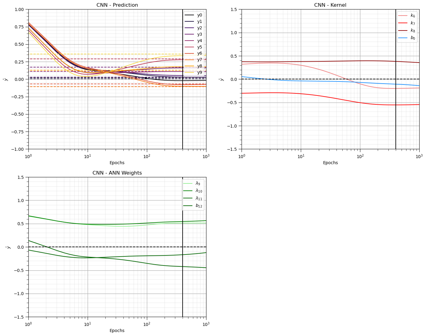
Now again we can visualize the model performance,
predictions over all training images vs. training epochs
model weights and biases vs. training epochs
plt.subplot(221)
for isample in range(0,nsample):
    plt.plot(np.arange(1,nepoch+1,1),yhat[:,isample],color=plt.cm.inferno(isample/nsample),label=r'y' + str(isample))
    plt.plot([0,nepoch],[ymat[isample],ymat[isample]],color=plt.cm.inferno(isample/nsample),ls='--')
plt.xlim([1,nepoch]); plt.ylim([-1,1])
plt.xlabel('Epochs'); plt.ylabel(r'$\hat{y}$'); plt.title('CNN - Prediction')
plt.vlines(400,-1.5,1.5,color='black')
add_grid(); plt.legend(loc='upper right'); plt.xscale('log')

plt.subplot(222)
plt.plot(np.arange(1,nepoch+1,1),w6,color='lightcoral',label = r'$k_6$')
plt.plot(np.arange(1,nepoch+1,1),w7,color='red',label = r'$k_7$')
plt.plot(np.arange(1,nepoch+1,1),w8,color='darkred',label = r'$k_8$')
plt.plot(np.arange(1,nepoch+1,1),bconv,color='dodgerblue',label = r'$b_0$')
plt.plot([1,nepoch],[0,0],color='black',ls='--')
plt.xlim([1,nepoch]); plt.ylim([-1.5,1.5]); plt.vlines(400,-1.5,1.5,color='black')
plt.xlabel('Epochs'); plt.ylabel(r'$\hat{y}$'); plt.title('CNN - Kernel')
add_grid(); plt.legend(loc='upper right'); plt.xscale('log')

plt.subplot(223)
plt.plot(np.arange(1,nepoch+1,1),w9,color='lightgreen',label = r'$\lambda_{9}$')
plt.plot(np.arange(1,nepoch+1,1),w10,color='green',label = r'$\lambda_{10}$')
plt.plot(np.arange(1,nepoch+1,1),w11,color='darkgreen',label = r'$\lambda_{11}$')
plt.plot(np.arange(1,nepoch+1,1),b12,color='darkgreen',label = r'$b_{12}$')
plt.plot([1,nepoch],[0,0],color='black',ls='--')
plt.xlim([1,nepoch]); plt.ylim([-1.5,1.5]); plt.vlines(400,-1.5,1.5,color='black')
plt.xlabel('Epochs'); plt.ylabel(r'$\hat{y}$'); plt.title('CNN - ANN Weights')
add_grid(); plt.legend(loc='upper right'); plt.xscale('log')


plt.subplots_adjust(left=0.0, bottom=0.0, right=2.0, top=2.1, wspace=0.2, hspace=0.2); plt.show()
About the Author#

Michael Pyrcz is a professor in the Cockrell School of Engineering, and the Jackson School of Geosciences, at The University of Texas at Austin, where he researches and teaches subsurface, spatial data analytics, geostatistics, and machine learning. Michael is also,
the principal investigator of the Energy Analytics freshmen research initiative and a core faculty in the Machine Learn Laboratory in the College of Natural Sciences, The University of Texas at Austin
an associate editor for Computers and Geosciences, and a board member for Mathematical Geosciences, the International Association for Mathematical Geosciences.
Michael has written over 70 peer-reviewed publications, a Python package for spatial data analytics, co-authored a textbook on spatial data analytics, Geostatistical Reservoir Modeling and author of two recently released e-books, Applied Geostatistics in Python: a Hands-on Guide with GeostatsPy and Applied Machine Learning in Python: a Hands-on Guide with Code.
All of Michael’s university lectures are available on his YouTube Channel with links to 100s of Python interactive dashboards and well-documented workflows in over 40 repositories on his GitHub account, to support any interested students and working professionals with evergreen content. To find out more about Michael’s work and shared educational resources visit his Website.
Want to Work Together?#
I hope this content is helpful to those that want to learn more about subsurface modeling, data analytics and machine learning. Students and working professionals are welcome to participate.
Want to invite me to visit your company for training, mentoring, project review, workflow design and / or consulting? I’d be happy to drop by and work with you!
Interested in partnering, supporting my graduate student research or my Subsurface Data Analytics and Machine Learning consortium (co-PI is Professor John Foster)? My research combines data analytics, stochastic modeling and machine learning theory with practice to develop novel methods and workflows to add value. We are solving challenging subsurface problems!
I can be reached at mpyrcz@austin.utexas.edu.
I’m always happy to discuss,
Michael
Michael Pyrcz, Ph.D., P.Eng. Professor, Cockrell School of Engineering and The Jackson School of Geosciences, The University of Texas at Austin
More Resources Available at: Twitter | GitHub | Website | GoogleScholar | Geostatistics Book | YouTube | Applied Geostats in Python e-book | Applied Machine Learning in Python e-book | LinkedIn
Comments#
This was a basic treatment of convolutional neural networks. Much more could be done and discussed, I have many more resources. Check out my shared resource inventory and the YouTube lecture links at the start of this chapter with resource links in the videos’ descriptions.
I hope this is helpful,
Michael