

Ridge Regression#
Michael J. Pyrcz, Professor, The University of Texas at Austin
Twitter | GitHub | Website | GoogleScholar | Geostatistics Book | YouTube | Applied Geostats in Python e-book | Applied Machine Learning in Python e-book | LinkedIn
Chapter of e-book “Applied Machine Learning in Python: a Hands-on Guide with Code”.
Cite this e-Book as:
Pyrcz, M.J., 2024, Applied Machine Learning in Python: A Hands-on Guide with Code [e-book]. Zenodo. doi:10.5281/zenodo.15169138 ![]()
The workflows in this book and more are available here:
Cite the MachineLearningDemos GitHub Repository as:
Pyrcz, M.J., 2024, MachineLearningDemos: Python Machine Learning Demonstration Workflows Repository (0.0.3) [Software]. Zenodo. DOI: 10.5281/zenodo.13835312. GitHub repository: GeostatsGuy/MachineLearningDemos ![]()
By Michael J. Pyrcz
© Copyright 2024.
This chapter is a tutorial for / demonstration of Ridge Regression.
YouTube Lecture: check out my lectures on:
These lectures are all part of my Machine Learning Course on YouTube with linked well-documented Python workflows and interactive dashboards. My goal is to share accessible, actionable, and repeatable educational content. If you want to know about my motivation, check out Michael’s Story.
Motivations for Ridge Regression#
Here’s a simple workflow, demonstration of ridge regression and comparison to linear regression for machine learning-based predictions. Why start with linear regression?
Linear regression is the simplest parametric predictive machine learning model
We learn about training machine learning models with an analytical solution calculated from the derivative of training MSE
Get’s us started with the concepts of loss functions and norms
We have access to analytics expressions for confidence intervals for model uncertainty and hypothesis tests for parameter significance
Why cover ridge regression next?
Some times linear regression is not simple enough and we actually need a simpler model!
Introduce the concept of model regularization and hyperparameter tuning
Here’s some basic details about predictive machine learning ridge regression models, let’s start with linear regression first and build to ridge regression:
Linear Regression#
Linear regression for prediction, let’s start by looking at a linear model fit to a set of data.
Let’s start by defining some terms,
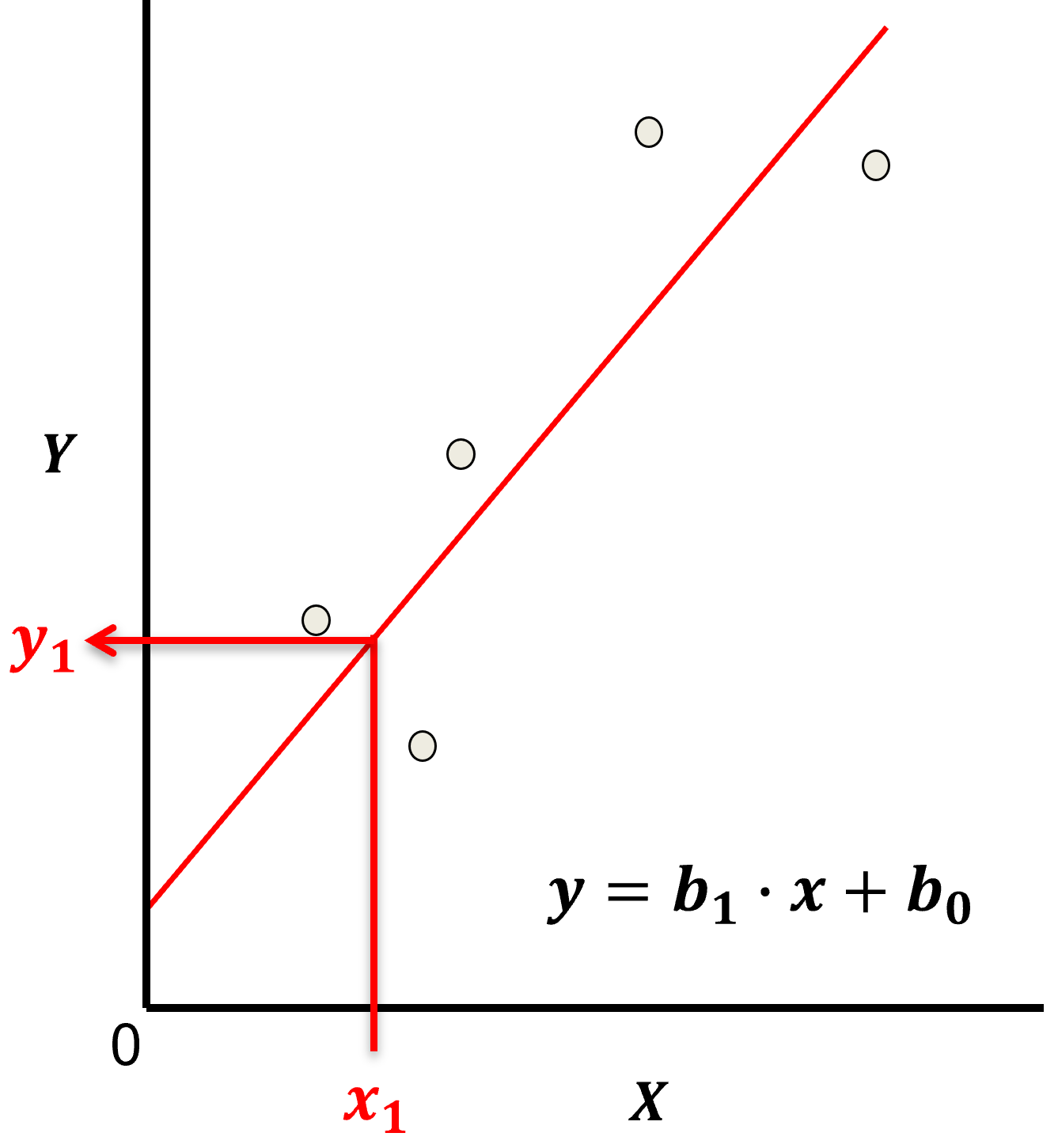
predictor feature - an input feature for the prediction model, given we are only discussing linear regression and not multilinear regression we have only one predictor feature, \(x\). On out plots (including above) the predictor feature is on the x-axis.
response feature - the output feature for the prediction model, in this case, \(y\). On our plots (including above) the response feature is on the y-axis.
Now, here are some key aspects of linear regression:
Parametric Model
This is a parametric predictive machine learning model, we accept an a prior assumption of linearity and then gain a very low parametric representation that is easy to train without a onerous amount of data.
the fit model is a simple weighted linear additive model based on all the available features, \(x_1,\ldots,x_m\).
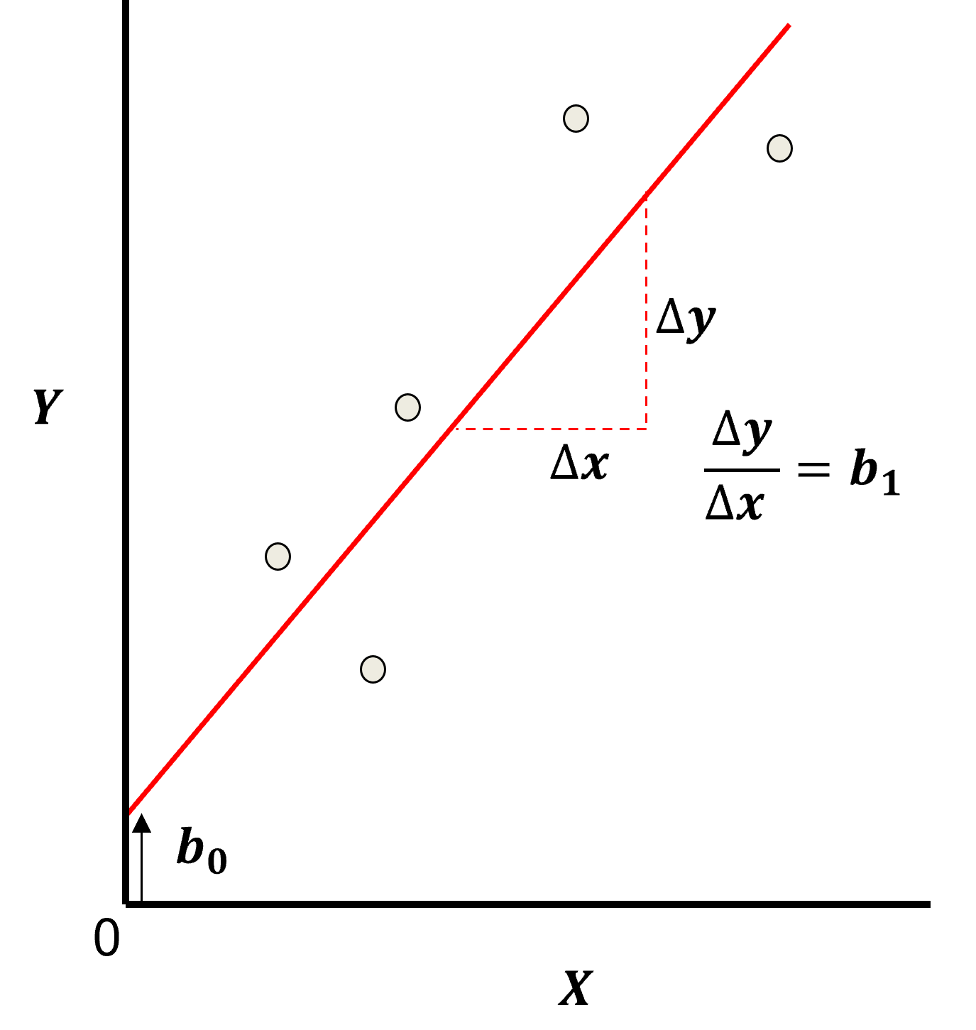
the parametric model takes the form of:
Here’s the visualization of the linear model parameters,
Least Squares
The analytical solution for the model parameters, \(b_1,\ldots,b_m,b_0\), is available for the L2 norm loss function, the errors are summed and squared known a least squares.
we minimize the error, residual sum of squares (RSS) over the training data:
where \(y_i\) is the actual response feature values and \(\sum_{\alpha = 1}^m b_{\alpha} x_{\alpha} + b_0\) are the model predictions, over the \(\alpha = 1,\ldots,n\) training data.
Here’s a visualization of the L2 norm loss function, MSE,
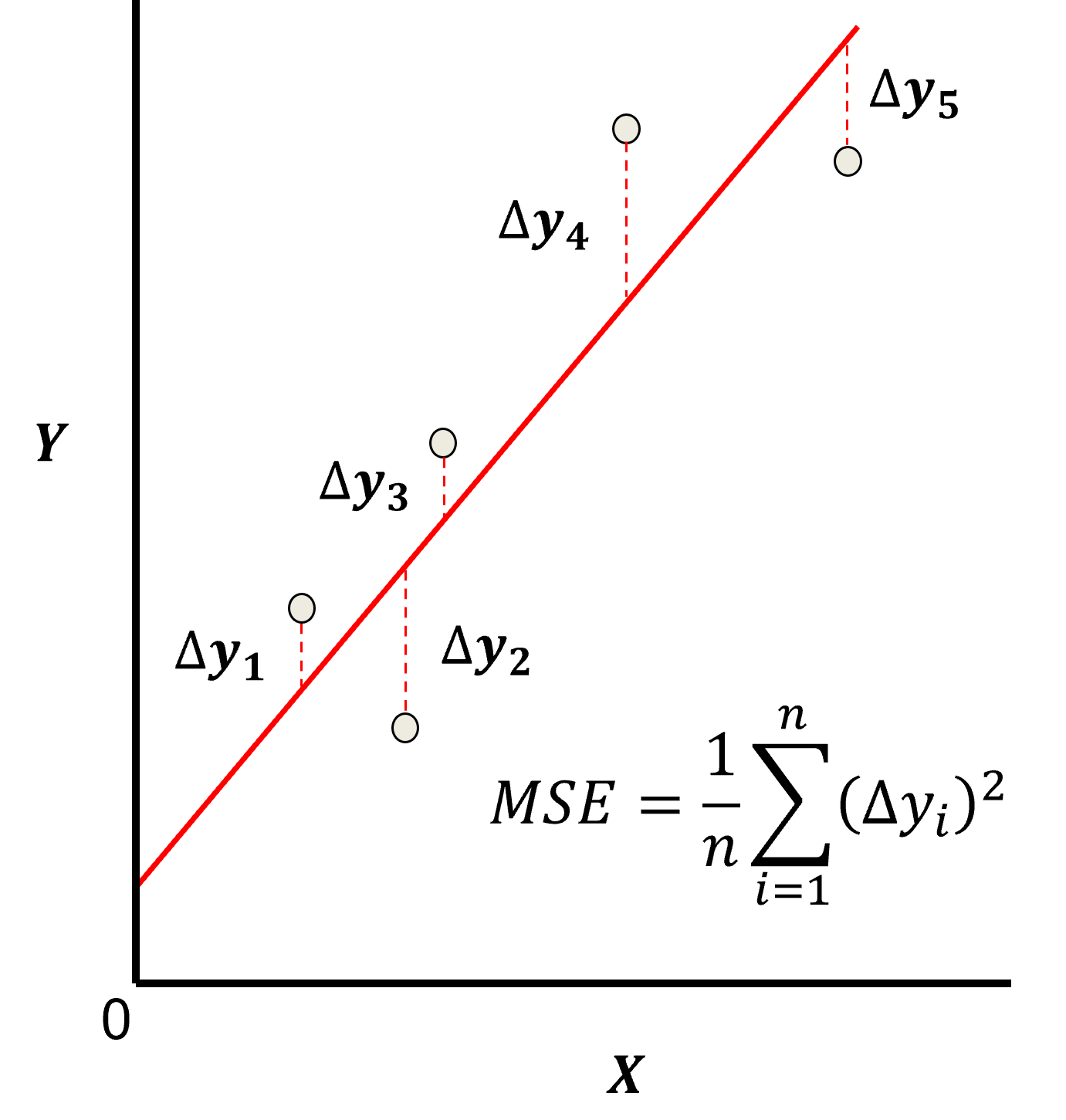
this may be simplified as the sum of square error over the training data,
\begin{equation} \sum_{i=1}^n (\Delta y_i)^2 \end{equation}
where \(\Delta y_i\) is actual response feature observation \(y_i\) minus the model prediction \(\sum_{\alpha = 1}^m b_{\alpha} x_{\alpha} + b_0\), over the \(i = 1,\ldots,n\) training data.
Assumptions
There are important assumption with our linear regression model,
Error-free - predictor variables are error free, not random variables
Linearity - response is linear combination of feature(s)
Constant Variance - error in response is constant over predictor(s) value
Independence of Error - error in response are uncorrelated with each other
No multicollinearity - none of the features are redundant with other features
Ridge Regression#
With ridge regression we add a hyperparameter, \(\lambda\), to our minimization, with a shrinkage penalty term, \(\sum_{j=1}^m b_{\alpha}^2\).
As a result, ridge regression training integrates two and often competing goals to find the model parameters,
find the model parameters that minimize the error with training data
minimize the slope parameters towards zero
Note: lambda does not include the intercept, \(b_0\).
The \(\lambda\) is a hyperparameter that controls the degree of fit of the model and may be related to the model bias-variance trade-off.
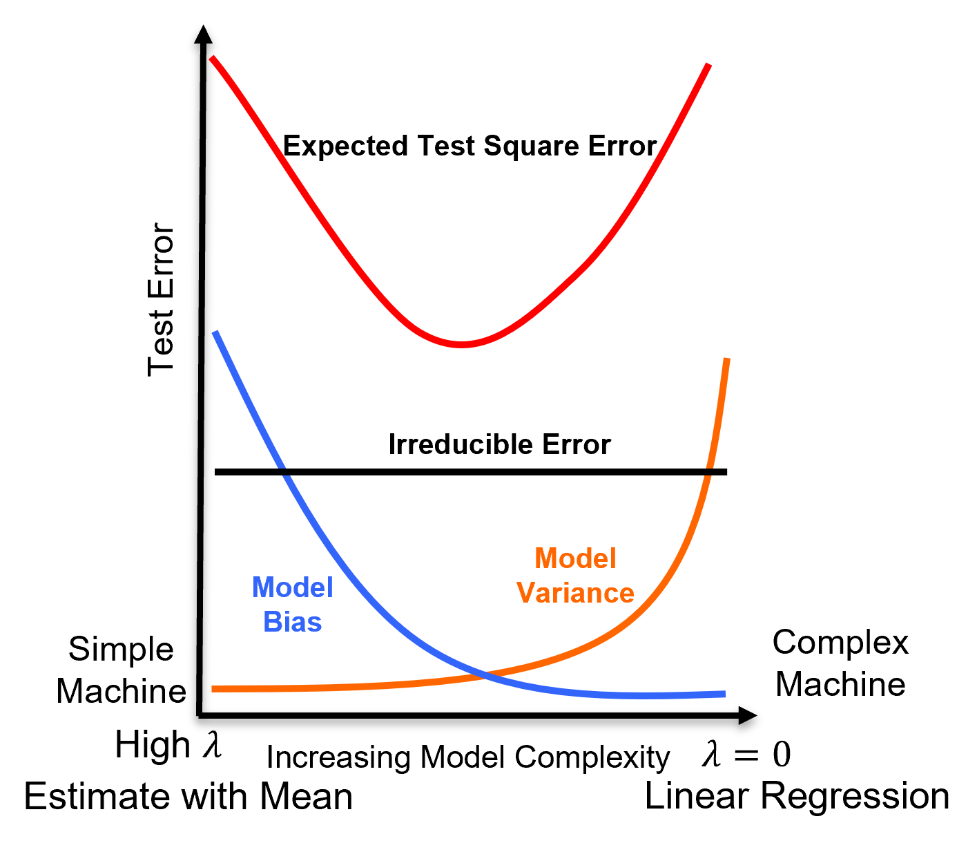
for \(\lambda \rightarrow 0\) the solution approaches linear regression, there is no bias (relative to a linear model fit), but the model variance is likely higher
as \(\lambda\) increases the model variance decreases and the model bias increases, the model becomes simpler
for \(\lambda \rightarrow \infty\) the model parameters \(b_1,\ldots,b_m\) shrink to 0.0 and the model predictions approaches the training data response feature mean
Here’s a variety of ridge regression models for various \(\lamda\) values that will be calculated in the workflow below,
Train / Test Data Split for Cross Validation-based Hyperparameter Tuning#
The available data is split into training and testing subsets.
in general 15-30% of the data is withheld from training to apply as testing data
testing data selection should be fair, the same difficulty of predictions (offset/different from the training data) Fair Train-test Split Paper (Salazar et al., 2022).
there are various other methods including train, validation and testing splits, and k-fold cross validation
Fundamentally, all these methods proceed by training models with training data and testing model accuracy over withheld testing data for a range of hyperparameters. Then the hyperparameters are selected that minimize error with the withheld testing dataset, this is hyperparameter tuning.
after hyperparameter tuning the model is retrained with all of the data with the selected hyperparameters.
the train, validation and testing approach then uses a 2nd withheld subset of the dataset to check the tuned model with data not applied for model training nor model tuning.
In the following workflow we will use the train and test approach for hyperparameter tuning. Here’s more details and a summary of the related concepts.
Model Parameter Training#
The training data is applied to train the model parameters such that the model minimizes mismatch with the training data
it is common to use mean square error (known as a L2 norm) as a loss function summarizing the model mismatch
minimizing the loss function for simple models an analytical solution may be available, but for most machine this requires an iterative optimization method to find the best model parameters
Here’s the derivation of the analytical solution, starting with the loss function with, least squares (left) and regularization (right) terms,
let’s convert this into matrix notation for convenience,
where \(\beta\) is a vector of the model parameters, \(y\) is a vector of response feature values, and \(X\) is a matrix of predictor feature values, both over the training data.
We can expand the quadratic term,
We take the partial derivative with respect to the model parameters and set it equal to 0.0,
Now we can further simplify with minor adjustments.
Divide both sides by 2,
Group the common terms,
where \(I\) is an identity matrix. Now we can solve for our ridge regression parameters,
Note, \(𝑋^𝑇 𝑋+\lambda I\) is generally invertible, so this is solvable.
This process is repeated over a range of model complexities specified by hyperparameters.
Interpretation of Regularization#
Another interpretation and motivation for ridge regression,
when \(𝑚 \ge 𝑛\), linear regression is ill-posed problem, i.e., a problem with more than 1 solution
for ill-posed problems we introduce some constraints or regularization to limit the solutions

Model Hyperparameter Tuning#
The withheld testing data is retrieved and loss function (usually the L2 norm again) is calculated to summarize the error over the testing data
this is repeated over the range of specified hyperparameters
the model complexity / hyperparameters that minimize the loss function / error summary in testing is selected
This is known are model hyperparameter tuning.
Model Overfit#
More model complexity / flexibility than can be justified with the available data, data accuracy, frequency and coverage
Model explains “idiosyncrasies” of the data, capturing data noise/error in the model
High accuracy in training, but low accuracy in testing / real-world use away from training data cases – poor ability of the model to generalize
If the model error in testing is increasing while the model error in training is decreasing, this is an indicator of an overfit model.
Load the Required Libraries#
We will also need some standard packages. These should have been installed with Anaconda 3.
%matplotlib inline
suppress_warnings = False
import os                                                     # to set current working directory
import os                                                     # to set current working directory
import numpy as np                                            # ndarrays and matrix math
import scipy.stats as st                                      # statistical methods
import pandas as pd                                           # DataFrames
import matplotlib.pyplot as plt                               # for plotting
from matplotlib.ticker import (MultipleLocator, AutoMinorLocator) # control of axes ticks
from sklearn.metrics import mean_squared_error, r2_score      # specific measures to check our models
from sklearn import linear_model                              # linear regression
from sklearn.linear_model import Ridge                        # ridge regression implemented in scikit learn
from sklearn.model_selection import cross_val_score           # multi-processor K-fold crossvalidation
from sklearn.model_selection import train_test_split          # train and test split
from IPython.display import display, HTML                     # custom displays
cmap = plt.cm.inferno                                         # default color bar, no bias and friendly for color vision defeciency
plt.rc('axes', axisbelow=True)                                # grid behind plotting elements
if suppress_warnings == True:
    import warnings                                           # supress any warnings for this demonstration
    warnings.filterwarnings('ignore')
If you get a package import error, you may have to first install some of these packages. This can usually be accomplished by opening up a command window on Windows and then typing ‘python -m pip install [package-name]’. More assistance is available with the respective package docs.
Declare Functions#
Let’s define a function to streamline the addition specified percentiles and major and minor gridlines to our plots.
def weighted_percentile(data, weights, perc):                 # calculate weighted percentile
    ix = np.argsort(data)
    data = data[ix]
    weights = weights[ix]
    cdf = (np.cumsum(weights) - 0.5 * weights) / np.sum(weights)
    return np.interp(perc, cdf, data)
# Function from iambr on StackOverflow @ https://stackoverflow.com/questions/21844024/weighted-percentile-using-numpy/32216049

def histogram_bounds(values,weights,color):                   # add uncertainty bounds to a histogram
    p10 = weighted_percentile(values,weights,0.1); avg = np.average(values,weights=weights); p90 = weighted_percentile(values,weights,0.9)
    plt.plot([p10,p10],[0.0,45],color = color,linestyle='dashed')
    plt.plot([avg,avg],[0.0,45],color = color)
    plt.plot([p90,p90],[0.0,45],color = color,linestyle='dashed')

def add_grid():
    plt.gca().grid(True, which='major',linewidth = 1.0); plt.gca().grid(True, which='minor',linewidth = 0.2) # add y grids
    plt.gca().tick_params(which='major',length=7); plt.gca().tick_params(which='minor', length=4)
    plt.gca().xaxis.set_minor_locator(AutoMinorLocator()); plt.gca().yaxis.set_minor_locator(AutoMinorLocator()) # turn on minor ticks

def display_sidebyside(*args):                                # display DataFrames side-by-side (ChatGPT 4.0 generated Spet, 2024)
    html_str = ''
    for df in args:
        html_str += df.head().to_html()  # Using .head() for the first few rows
    display(HTML(f'<div style="display: flex;">{html_str}</div>'))
Set the Working Directory#
I always like to do this so I don’t lose files and to simplify subsequent read and writes (avoid including the full address each time). Also, in this case make sure to place the required (see below) data file in this working directory.
#os.chdir("C:\PGE337") # set the working directory
You will have to update the part in quotes with your own working directory and the format is different on a Mac (e.g. “~/PGE”).
Loading Tabular Data#
Here’s the command to load our comma delimited data file in to a Pandas’ DataFrame object.
Let’s load the provided multivariate, spatial dataset ‘unconv_MV.csv’. This dataset has variables from 1,000 unconventional wells including:
density (\(g/cm^{3}\))
porosity (volume %)
Note, the dataset is synthetic.
We load it with the pandas ‘read_csv’ function into a DataFrame we called ‘my_data’ and then preview it to make sure it loaded correctly.
add_error = True                                              # add random error to the response feature
std_error = 1.0; seed = 71071

yname = 'Porosity'; xname = 'Density'                         # specify the predictor features (x2) and response feature (x1)
xmin = 1.0; xmax = 2.5                                        # set minimums and maximums for visualization
ymin = 0.0; ymax = 25.0
xlabel = 'Porosity'; ylabel = 'Density'                       # specify the feature labels for plotting
yunit = '%'; xunit = '$g/cm^{3}$'
Xlabelunit = xlabel + ' (' + xunit + ')'
ylabelunit = ylabel + ' (' + yunit + ')'

#df = pd.read_csv("Density_Por_data.csv")                     # load the data from local current directory
df = pd.read_csv(r"https://raw.githubusercontent.com/GeostatsGuy/GeoDataSets/master/Density_Por_data.csv") # load the data from my github repo
df = df.sample(frac=1.0, random_state = 73073); df = df.reset_index() # extract 30% random to reduce the number of data

if add_error == True:                                         # method to add error
    np.random.seed(seed=seed)                                 # set random number seed
    df[yname] = df[yname] + np.random.normal(loc = 0.0,scale=std_error,size=len(df)) # add noise
    values = df._get_numeric_data(); values[values < 0] = 0   # set negative to 0 in a shallow copy ndarray
Train-Test Split#
For simplicity we apply a random train-test split with the train_test_split function from scikit-learn package, model_selection module.
x_train, x_test, y_train, y_test = train_test_split(df[xname],df[yname],test_size=0.25,random_state=73073) # train and test split
# y_train = pd.DataFrame({yname:y_train.values}); y_test = pd.DataFrame({yname:y_test.values}) # optional to ensure response is a DataFrame

y = df[yname].values.reshape(len(df))                         # features as 1D vectors
x = df[xname].values.reshape(len(df))

df_train = pd.concat([x_train,y_train],axis=1)                # features as train and test DataFrames
df_test = pd.concat([x_test,y_test],axis=1)
Visualize the DataFrame#
Visualizing the DataFrame is useful first check of the data.
many things can go wrong, e.g., we loaded the wrong data, all the features did not load, etc.
We can preview by utilizing the ‘head’ DataFrame member function (with a nice and clean format, see below).
we have a custom function to preview the training and testing DataFrames side-by-side.
print('   Training DataFrame      Testing DataFrame')
display_sidebyside(df_train,df_test)
Training DataFrame Testing DataFrame
| Density | Porosity | |
|---|---|---|
| 24 | 1.778580 | 11.426485 |
| 101 | 2.410560 | 8.488544 |
| 88 | 2.216014 | 10.133693 |
| 79 | 1.631896 | 12.712326 |
| 58 | 1.528019 | 16.129542 |
| Density | Porosity | |
|---|---|---|
| 59 | 1.742534 | 15.380154 |
| 1 | 1.404932 | 13.710628 |
| 35 | 1.552713 | 14.131878 |
| 92 | 1.762359 | 11.154896 |
| 22 | 1.885087 | 9.403056 |
Summary Statistics for Tabular Data#
There are a lot of efficient methods to calculate summary statistics from tabular data in DataFrames. The describe command provides count, mean, minimum, maximum in a nice data table.
print('     Training DataFrame         Testing DataFrame')
display_sidebyside(df_train.describe().loc[['count', 'mean', 'std', 'min', 'max']],df_test.describe().loc[['count', 'mean', 'std', 'min', 'max']])
Training DataFrame Testing DataFrame
| Density | Porosity | |
|---|---|---|
| count | 78.000000 | 78.000000 |
| mean | 1.739027 | 12.501465 |
| std | 0.302510 | 3.428260 |
| min | 0.996736 | 3.276449 |
| max | 2.410560 | 21.660179 |
| Density | Porosity | |
|---|---|---|
| count | 27.000000 | 27.000000 |
| mean | 1.734710 | 12.380796 |
| std | 0.247761 | 2.916045 |
| min | 1.067960 | 7.894595 |
| max | 2.119652 | 18.133771 |
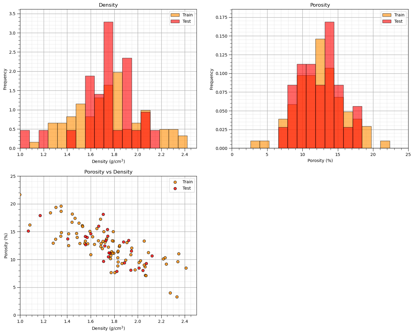
Visualize the Data#
Let’s check the consistency and coverage of training and testing with histograms and scatter plots.
check to make sure the train and test data cover the range of possible feature combinations
ensure we are not extrapolating beyond the training data with the testing cases
nbins = 20                                                    # number of histogram bins

plt.subplot(221)
freq1,_,_ = plt.hist(x=df_train[xname],weights=None,bins=np.linspace(xmin,xmax,nbins),alpha = 0.6,
                     edgecolor='black',color='darkorange',density=True,label='Train')
freq2,_,_ = plt.hist(x=df_test[xname],weights=None,bins=np.linspace(xmin,xmax,nbins),alpha = 0.6,
                     edgecolor='black',color='red',density=True,label='Test')
max_freq = max(freq1.max()*1.10,freq2.max()*1.10)
plt.xlabel(xname + ' (' + xunit + ')'); plt.ylabel('Frequency'); plt.ylim([0.0,max_freq]); plt.title('Density'); add_grid()
plt.xlim([xmin,xmax]); plt.legend(loc='upper right')

plt.subplot(222)
freq1,_,_ = plt.hist(x=df_train[yname],weights=None,bins=np.linspace(ymin,ymax,nbins),alpha = 0.6,
                     edgecolor='black',color='darkorange',density=True,label='Train')
freq2,_,_ = plt.hist(x=df_test[yname],weights=None,bins=np.linspace(ymin,ymax,nbins),alpha = 0.6,
                     edgecolor='black',color='red',density=True,label='Test')
max_freq = max(freq1.max()*1.10,freq2.max()*1.10)
plt.xlabel(yname + ' (' + yunit + ')'); plt.ylabel('Frequency'); plt.ylim([0.0,max_freq]); plt.title('Porosity'); add_grid()
plt.xlim([ymin,ymax]); plt.legend(loc='upper right')

plt.subplot(223)                                              # plot the model
plt.scatter(df_train[xname],df_train[yname],s=40,marker='o',color = 'darkorange',alpha = 0.8,edgecolor = 'black',zorder=10,label='Train')
plt.scatter(df_test[xname],df_test[yname],s=40,marker='o',color = 'red',alpha = 0.8,edgecolor = 'black',zorder=10,label='Test')
plt.title('Porosity vs Density')
plt.xlabel(xname + ' (' + xunit + ')')
plt.ylabel(yname + ' (' + yunit + ')')
plt.legend(); add_grid(); plt.xlim([xmin,xmax]); plt.ylim([ymin,ymax])

plt.subplots_adjust(left=0.0, bottom=0.0, right=2.0, top=2.1, wspace=0.2, hspace=0.2)
#plt.savefig('Test.pdf', dpi=600, bbox_inches = 'tight',format='pdf')
plt.show()
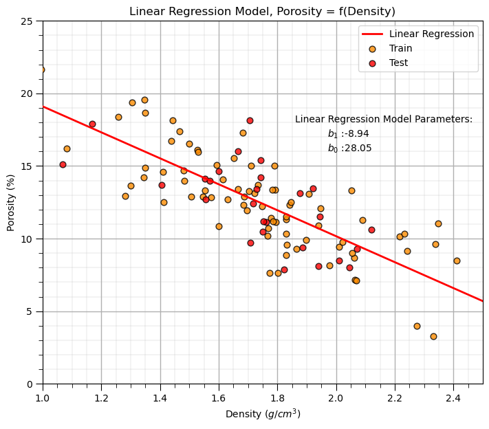
Linear Regression Model#
Let’s first calculate the linear regression model. We use scikit learn and then extend the same workflow to ridge regression.
we are building a model, \(\phi = f(\rho)\), where \(\phi\) is porosity and \(\rho\) is density.
we could also say, we have “porosity regressed on density”.
Our model has this specific equation,
linear_reg = linear_model.LinearRegression()                  # instantiate the model

linear_reg.fit(df_train[xname].values.reshape(len(df_train),1), df_train[yname]) # train the model parameters
x_model = np.linspace(xmin,xmax,10)
y_model_linear = linear_reg.predict(x_model.reshape(-1, 1))   # predict at the withheld test data

plt.subplot(111)                                              # plot the data, model with model parameters
plt.plot(x_model,y_model_linear, color='red', linewidth=2,label='Linear Regression',zorder=100)
plt.scatter(df_train[xname],df_train[yname],s=40,marker='o',color = 'darkorange',alpha = 0.8,edgecolor = 'black',zorder=10,label='Train')
plt.scatter(df_test[xname],df_test[yname],s=40,marker='o',color = 'red',alpha = 0.8,edgecolor = 'black',zorder=10,label='Test')
plt.annotate('Linear Regression Model Parameters:',[1.86,18]) # add the model to the plot
plt.annotate(r'$b_1$ :' + str(np.round(linear_reg.coef_ [0],2)),[1.97,17])
plt.annotate(r'$b_0$ :' + str(np.round(linear_reg.intercept_,2)),[1.97,16])
plt.title('Linear Regression Model, Porosity = f(Density)')
plt.xlabel(xname + ' (' + xunit + ')')
plt.ylabel(yname + ' (' + yunit + ')')
plt.legend(loc='upper right'); add_grid(); plt.xlim([xmin,xmax]); plt.ylim([ymin,ymax])

plt.subplots_adjust(left=0.0, bottom=0.0, right=1.0, top=1.1, wspace=0.2, hspace=0.2); plt.show()
You may have noticed the additional reshape operation applied to the predictor feature in the predict function.
y_linear_model = linear_reg.predict(x_model.reshape(-1, 1)) # predict at the withheld test data
This is needed because scikit-learn assumes more than one predictor feature; therefore, expects a 2D array of samples (rows) and features (columns), but we have only a 1D vector.
the reshape operation turns the 1D vector into a 2D vector with only 1 column
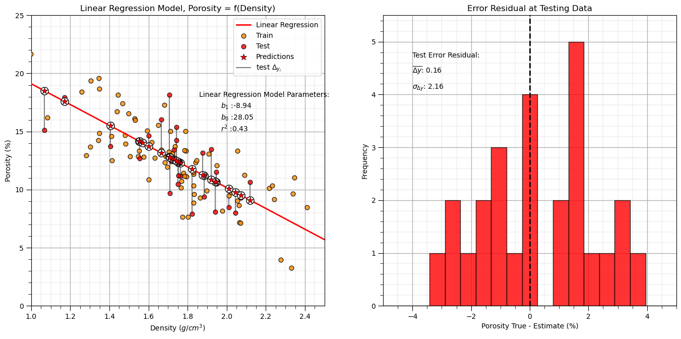
Linear Regression Model Checks#
Let’s run some quick model checks. Much more could be done, but I limit this for brevity here.
see the Linear Regression chapter for more information and checks
y_pred_linear = linear_reg.predict(df_test[xname].values.reshape(len(df_test),1)) # predict at test data
r_squared_linear = r2_score(df_test[yname].values, y_pred_linear)

plt.subplot(121)                                              # plot testing diagnostics
plt.plot(x_model,y_model_linear, color='red', linewidth=2,label='Linear Regression',zorder=100)
plt.scatter(df_train[xname],df_train[yname],s=40,marker='o',color = 'darkorange',alpha = 0.8,edgecolor = 'black',zorder=10,label='Train')
plt.scatter(df_test[xname],df_test[yname],s=40,marker='o',color = 'red',alpha = 0.8,edgecolor = 'black',zorder=10,label='Test')
# plt.scatter(df_test[xname], y_pred,color='grey',edgecolor='black',s = 40, alpha = 1.0, label = 'predictions',zorder=100)
plt.scatter(df_test[xname], y_pred_linear,color='white',s=120,marker='o',linewidths=1.0, edgecolors="black",zorder=300)
plt.scatter(df_test[xname], y_pred_linear,color='red',s=90,marker='*',linewidths=0.5, edgecolors="black",zorder=320,label='Predictions')

for idata in range(0,len(df_test)):
    if idata == 0:
        plt.plot([df_test.iloc[idata][xname],df_test.iloc[idata][xname]],[df_test.iloc[idata][yname],
                        y_pred_linear[idata]],color='grey',label=r'test $\Delta_{y_i}$',zorder=1)
    else:
        plt.plot([df_test.iloc[idata][xname],df_test.iloc[idata][xname]],[df_test.iloc[idata][yname],
                        y_pred_linear[idata]],color='grey',zorder=1)

plt.annotate('Linear Regression Model Parameters:',[1.86,18]) # add the model to the plot
plt.annotate(r'$b_1$ :' + str(np.round(linear_reg.coef_ [0],2)),[1.97,17])
plt.annotate(r'$b_0$ :' + str(np.round(linear_reg.intercept_,2)),[1.97,16])
plt.annotate(r'$r^2$ :' + str(np.round(r_squared_linear,2)),[1.97,15])
plt.title('Linear Regression Model, Porosity = f(Density)')
plt.xlabel(xname + ' (' + xunit + ')')
plt.ylabel(yname + ' (' + yunit + ')')
plt.legend(loc='upper right'); add_grid(); plt.xlim([xmin,xmax]); plt.ylim([ymin,ymax])

y_res_linear = y_pred_linear - df_test['Porosity'].values     # calculate the test residual

plt.subplot(122)
plt.hist(y_res_linear, color = 'red', alpha = 0.8, edgecolor = 'black', bins = np.linspace(-5,5,20))
plt.title("Error Residual at Testing Data"); plt.xlabel(yname + ' True - Estimate (%)');plt.ylabel('Frequency')
plt.vlines(0,0,5.5,color='black',ls='--',lw=2)
plt.annotate('Test Error Residual:',[-4,4.7]) # add residual summary statistics
plt.annotate(r'$\overline{\Delta{y}}$: ' + str(round(np.average(y_res_linear),2)),[-4,4.4])
plt.annotate(r'$\sigma_{\Delta{y}}$: ' + str(np.round(np.std(y_res_linear),2)),[-4,4.1])
add_grid(); plt.xlim(-5,5); plt.ylim(0,5.5)

plt.subplots_adjust(left=0.0, bottom=0.0, right=2.0, top=1.2, wspace=0.2, hspace=0.2); plt.show()
Ridge Regression Model#
Let’s replace the scikit-learn linear regression method with the scikit-learn ridge regression method.
note, we must now set the \(\lambda\) hyperparameter.
in scikit-learn the hyperparameter(s) is(are) set with the instantiation of the model
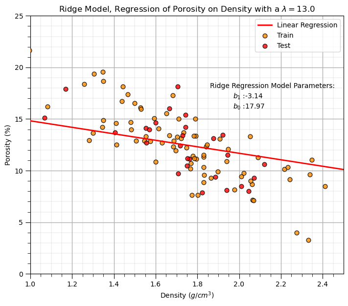
lam = 13.0                                                     # lambda hyperparameter

ridge_reg = Ridge(alpha=lam)                                  # instantiate the model

ridge_reg.fit(df_train[xname].values.reshape(len(df_train),1), df_train[yname]) # train the model parameters
x_model = np.linspace(xmin,xmax,10)
y_model_ridge = ridge_reg.predict(x_model.reshape(10,1))      # predict with the fit model

plt.subplot(111)                                              # plot the data, model with model parameters
plt.plot(x_model,y_model_ridge, color='red', linewidth=2,label='Linear Regression',zorder=100)
plt.scatter(df_train[xname],df_train[yname],s=40,marker='o',color = 'darkorange',alpha = 0.8,edgecolor = 'black',zorder=10,label='Train')
plt.scatter(df_test[xname],df_test[yname],s=40,marker='o',color = 'red',alpha = 0.8,edgecolor = 'black',zorder=10,label='Test')
plt.annotate('Ridge Regression Model Parameters:',[1.86,18]) # add the model to the plot
plt.annotate(r'$b_1$ :' + str(np.round(ridge_reg.coef_ [0],2)),[1.97,17])
plt.annotate(r'$b_0$ :' + str(np.round(ridge_reg.intercept_,2)),[1.97,16])
plt.title('Ridge Model, Regression of ' + yname + ' on ' + xname + r' with a $\lambda = $' + str(lam))
plt.xlabel(xname + ' (' + xunit + ')')
plt.ylabel(yname + ' (' + yunit + ')')
plt.legend(loc='upper right'); add_grid(); plt.xlim([xmin,xmax]); plt.ylim([ymin,ymax])

plt.subplots_adjust(left=0.0, bottom=0.0, right=1.0, top=1.1, wspace=0.2, hspace=0.2); plt.show()
Let’s repeat the simple model checks that we applied with our linear regression model.
y_pred_ridge = ridge_reg.predict(df_test[xname].values.reshape(len(df_test),1)) # predict at test data
r_squared = r2_score(df_test[yname].values, y_pred_ridge)

plt.subplot(121)                                              # plot testing diagnostics
plt.plot(x_model,y_model_ridge, color='red', linewidth=2,label='Linear Regression',zorder=100)
plt.scatter(df_train[xname],df_train[yname],s=40,marker='o',color = 'darkorange',alpha = 0.8,edgecolor = 'black',zorder=10,label='train')
plt.scatter(df_test[xname],df_test[yname],s=40,marker='o',color = 'red',alpha = 0.8,edgecolor = 'black',zorder=10,label='test')
plt.scatter(df_test[xname], y_pred_ridge,color='white',s=120,marker='o',linewidths=1.0, edgecolors="black",zorder=300)
plt.scatter(df_test[xname], y_pred_ridge,color='red',s=90,marker='*',linewidths=0.5, edgecolors="black",zorder=320,label='predictions')

for idata in range(0,len(df_test)):
    if idata == 0:
        plt.plot([df_test.iloc[idata][xname],df_test.iloc[idata][xname]],[df_test.iloc[idata][yname],
                        y_pred_ridge[idata]],color='grey',label=r'test $\Delta_{y_i}$',zorder=1)
    else:
        plt.plot([df_test.iloc[idata][xname],df_test.iloc[idata][xname]],[df_test.iloc[idata][yname],
                        y_pred_ridge[idata]],color='grey',zorder=1)

plt.annotate('Ridge Regression Model Parameters:',[1.81,18]) # add the model to the plot
plt.annotate(r'$b_1$ :' + str(np.round(ridge_reg.coef_ [0],2)),[1.97,17])
plt.annotate(r'$b_0$ :' + str(np.round(ridge_reg.intercept_,2)),[1.97,16])
plt.title('Ridge Model, Regression of ' + yname + ' on ' + xname + r' with a $\lambda = $' + str(lam))
plt.xlabel(xname + ' (' + xunit + ')')
plt.ylabel(yname + ' (' + yunit + ')')
plt.legend(loc='upper right'); add_grid(); plt.xlim([xmin,xmax]); plt.ylim([ymin,ymax])

y_res_ridge = y_pred_ridge - df_test['Porosity'].values       # calculate the test residual

plt.subplot(122)
plt.hist(y_res_ridge, color = 'red', alpha = 0.8, edgecolor = 'black', bins = np.linspace(-5,5,20))
plt.title("Error Residual at Testing Data"); plt.xlabel(yname + ' True - Estimate (%)');plt.ylabel('Frequency')
plt.vlines(0,0,5.5,color='red',lw=2,zorder=1); plt.vlines(np.average(y_res_ridge),0,5.5,color='black',ls='--',zorder=10)
plt.annotate('Residual Average = ' + str(np.round(np.average(y_res_ridge),2)),[np.average(y_res_ridge)+0.2,2.5],rotation=90.0)
plt.annotate('Test Error Residual:',[-4,4.7]) # add residual summary statistics
plt.annotate(r'$\overline{\Delta{y}}$: ' + str(round(np.average(y_res_ridge),2)),[-4,4.4])
plt.annotate(r'$\sigma_{\Delta{y}}$: ' + str(np.round(np.std(y_res_ridge),2)),[-4,4.1])
add_grid(); plt.xlim(-5,5); plt.ylim(0,5.5)

plt.subplots_adjust(left=0.0, bottom=0.0, right=2.0, top=1.1, wspace=0.2, hspace=0.2); plt.show()
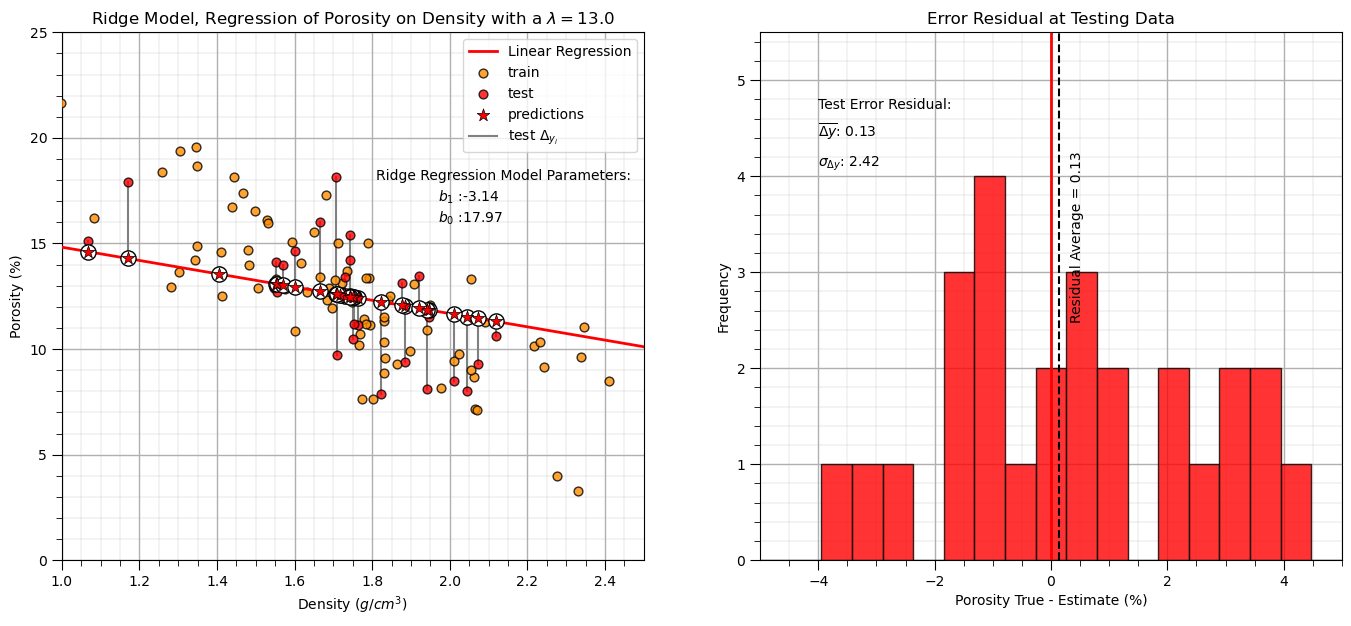
Interesting, we explained less variance and have a larger residual standard deviation (more error).
ridge regression for our arbitrarily selected hyperparameter, \(\lambda\), actually reduced both testing variance explained and accuracy
this is not surprising, we are not actually tuning the hyperparameter to get the best model!
Investigating the Lambda Hyperparameter#
Let’s loop over multiple lambda values - from 0 to 100 and observe the change in:
training and testing, mean square error (MSE) and variance explained
# Arrays to store the results
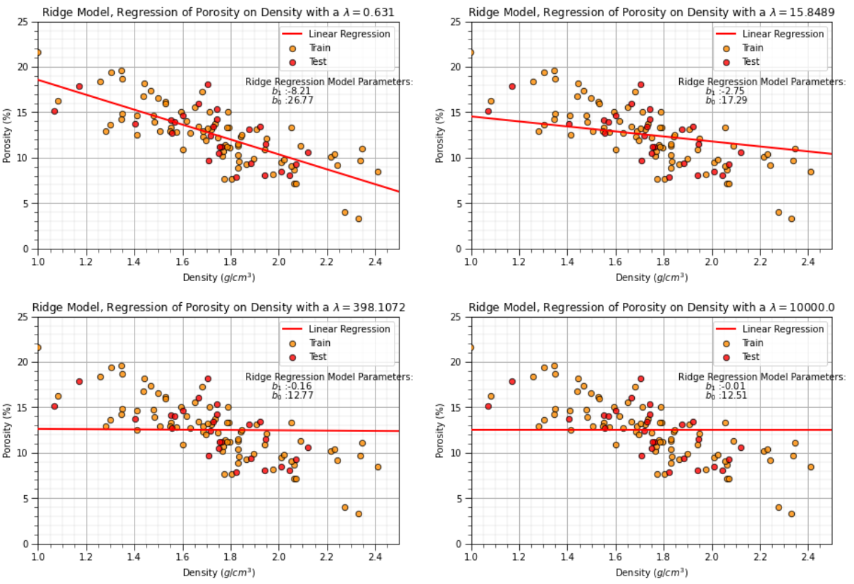
ncases = 6
lamd_mat = np.logspace(-3,4,ncases)
x_model = np.linspace(xmin,xmax,10)
var_explained_train = np.zeros(ncases); var_explained_test = np.zeros(ncases)
mse_train = np.zeros(ncases); mse_test = np.zeros(ncases)
for ilam in range(0,len(lamd_mat)): # Loop over all lambda values
ridge_reg = Ridge(alpha=lamd_mat[ilam])
ridge_reg.fit(df_train[xname].values.reshape(len(df_train),1), df_train[yname]) # fit model
y_model = ridge_reg.predict(x_model.reshape(10,1)) # predict with the fit model
y_pred_train = ridge_reg.predict(df_train[xname].values.reshape(len(df_train),1)) # predict with the fit model
var_explained_train[ilam] = r2_score(df_train[yname].values, y_pred_train)
mse_train[ilam] = mean_squared_error(df_train[yname].values, y_pred_train)
y_pred_test = ridge_reg.predict(df_test[xname].values.reshape(len(df_test),1))
var_explained_test[ilam] = r2_score(df_test[yname].values, y_pred_test)
mse_test[ilam] = mean_squared_error(df_test[yname].values, y_pred_test)
if ilam <= 7:
plt.subplot(4,2,ilam+1)
plt.plot(x_model,y_model, color='red', linewidth=2,label='Linear Regression',zorder=100)
plt.scatter(df_train[xname],df_train[yname],s=40,marker='o',color = 'darkorange',alpha = 0.8,edgecolor = 'black',zorder=10,label='Train')
plt.scatter(df_test[xname],df_test[yname],s=40,marker='o',color = 'red',alpha = 0.8,edgecolor = 'black',zorder=10,label='Test')
plt.annotate('Ridge Regression Model Parameters:',[1.86,18]) # add the model to the plot
plt.annotate(r'$b_1$ :' + str(np.round(ridge_reg.coef_ [0],2)),[1.97,17])
plt.annotate(r'$b_0$ :' + str(np.round(ridge_reg.intercept_,2)),[1.97,16])
plt.title('Ridge Model, Regression of ' + yname + ' on ' + xname + r' with a $\lambda = $' + str(round(lamd_mat[ilam],4)))
plt.xlabel(xname + ' (' + xunit + ')')
plt.ylabel(yname + ' (' + yunit + ')')
plt.legend(loc='upper right'); add_grid(); plt.xlim([xmin,xmax]); plt.ylim([ymin,ymax])
plt.subplots_adjust(left=0.0, bottom=0.0, right=2.0, top=4.2, wspace=0.2, hspace=0.2); plt.show()
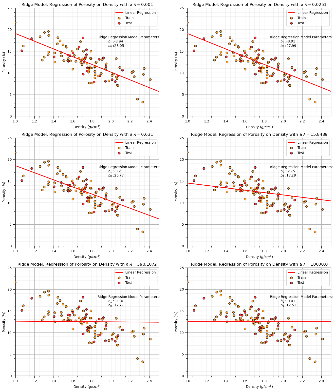
We can observe from the first 8 cases above of the trained ridge regression model that increase in the \(\lambda\) hyperparameter decreases the slope of the linear fit.
Let’s plot the mean squaure error and variance explained over train and test datasets.
Recall, the variance explained, \(R^2\) , is given by,
where \(SS_{\text{residual}}\) is the sum of squares of residuals (or errors), and \(SS_{\text{total}}\) is the total sum of squares (the variance of the observed data).
and the Mean Squared Error (MSE) is given by,
where \(y_i\) is the actual value, \(\hat{y}_i\) is the predicted value, and \(n\) is the number of data points.
ncases = 100
lamd_mat = np.logspace(-3,4,ncases)
x_model = np.linspace(xmin,xmax,10)
var_explained_train = np.zeros(ncases); var_explained_test = np.zeros(ncases)
mse_train = np.zeros(ncases); mse_test = np.zeros(ncases)

for ilam in range(0,len(lamd_mat)):                           # Loop over all lambda values
    ridge_reg = Ridge(alpha=lamd_mat[ilam])
    ridge_reg.fit(df_train[xname].values.reshape(len(df_train),1), df_train[yname]) # fit model

    y_model = ridge_reg.predict(x_model.reshape(10,1))        # predict with the fit model
    y_pred_train = ridge_reg.predict(df_train[xname].values.reshape(len(df_train),1)) # predict with the fit model
    var_explained_train[ilam] = r2_score(df_train[yname].values, y_pred_train)
    mse_train[ilam] = mean_squared_error(df_train[yname].values, y_pred_train)

    y_pred_test = ridge_reg.predict(df_test[xname].values.reshape(len(df_test),1))
    var_explained_test[ilam] = r2_score(df_test[yname].values, y_pred_test)
    mse_test[ilam] = mean_squared_error(df_test[yname].values, y_pred_test)

plt.subplot(121)
plt.plot(lamd_mat, var_explained_train,  color='darkorange', linewidth = 2, label = 'Train')
plt.plot(lamd_mat, var_explained_test,  color='red', linewidth = 2, label = 'Test')
plt.title('Variance Explained vs. Lambda'); plt.xlabel('Lambda'); plt.ylabel('Variance Explained')
plt.xlim(0.001,10000.); plt.xscale('log'); plt.ylim(0,1.0);
plt.grid(True); plt.minorticks_on(); plt.grid(which='minor', linestyle=':', linewidth=0.5); plt.legend()

plt.subplot(122)
plt.plot(lamd_mat, mse_train,  color='darkorange', linewidth = 2, label = 'Train')
plt.plot(lamd_mat, mse_test,  color='red', linewidth = 2, label = 'Test')
plt.title('MSE vs. Lambda'); plt.xlabel('Lambda'); plt.ylabel('Mean Square Error')
plt.xlim(0.001,10000.); plt.xscale('log'); plt.ylim(0,15.0); plt.legend()
plt.grid(True); plt.minorticks_on(); plt.grid(which='minor', linestyle=':', linewidth=0.5); plt.legend()

plt.subplots_adjust(left=0.0, bottom=0.0, right=2.0, top=1.2, wspace=0.2, hspace=0.3); plt.show()
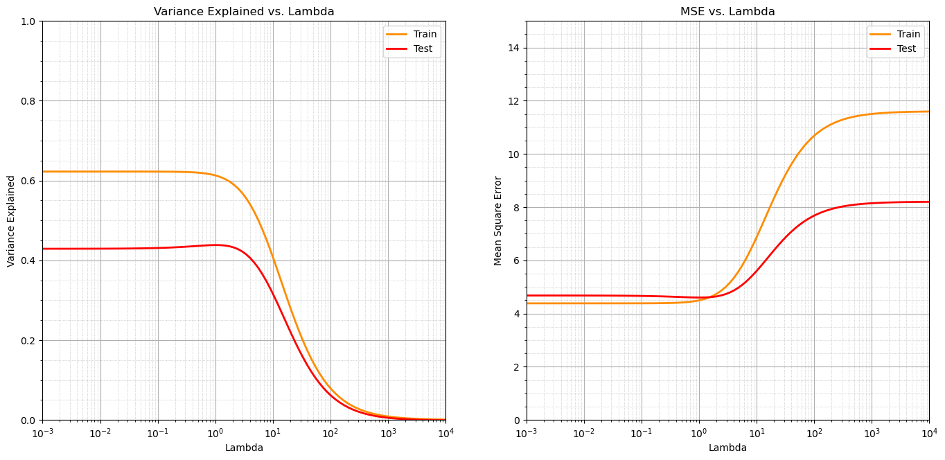
We observe that as we increase the lambda parameter the variance explained decreases and the mean square error increases.
this makes sense as the data has a consistent linear trend and as the slope ‘shrinks’ to zero the error increases and the variance explained decreases
there could be other cases where the reduced slope actually performs better in testing. For example with sparse and noisy data.
Model Variance#
Now let’s explore the concept of model variance, an important part of machine learning accuracy in testing.
the sensitivity of the model to the specific training data
as \(\lambda\) increases the sensitivity to the training data, model variance decreases
Let’s demonstrate this with this workflow:
loop over multiple lambda values
loop over multiple bootstrap samples of the data
calculate the ridge regression fit (slope)
calculate the variance of these bootstrap results
WARNING: this will take several minutes to run
L = 200                                                       # the number of bootstrap realizations

nsamples = 20                                                 # the number of samples in each bootstrap realization
nlambda = 100                                                 # number of lambda values to evaluate

coef_mat = np.zeros(L)                                        # declare arrays to store the results
variance_coef = np.zeros(nlambda)

#lamd_mat = np.linspace(0.0,100.0,nlambda)
lambda_mat = np.logspace(-2,5,nlambda)
for ilam in range(0,len(lambda_mat)):                         # loop over all lambda values
    for l in range(0, L):                                     # loop over all bootstrap realizations
        df_sample = df.sample(n = nsamples)                   # random sample (1 bootstrap)
        ridge_reg = Ridge(alpha=lambda_mat[ilam])             # instantiate model
        ridge_reg.fit(df_sample[xname].values.reshape(nsamples,1), df_sample[yname]) # fit model
        coef_mat[l] = ridge_reg.coef_[0]                      # get the slope parameter
    variance_coef[ilam] = np.var(coef_mat)                    # calculate the variance of the slopes over the L bootstraps

plt.subplot(111)
plt.plot(lambda_mat, variance_coef,  color='black', linewidth = 3, label = 'Slope Variance')
plt.title('Model Variance vs. Lambda Hyperparameter'); plt.xlabel('Lambda'); plt.ylabel('Model Variance - Variance of the Slope Parameter, $b_1$')
plt.xlim(0.01,100000.); plt.ylim(0.0,5.0); plt.xscale('log')
plt.subplots_adjust(left=0.0, bottom=0.0, right=2.0, top=1.0, wspace=0.2, hspace=0.2)
plt.grid(which='both')
plt.subplots_adjust(left=0.0, bottom=0.0, right=2.0, top=1.0, wspace=0.2, hspace=0.2); plt.show()
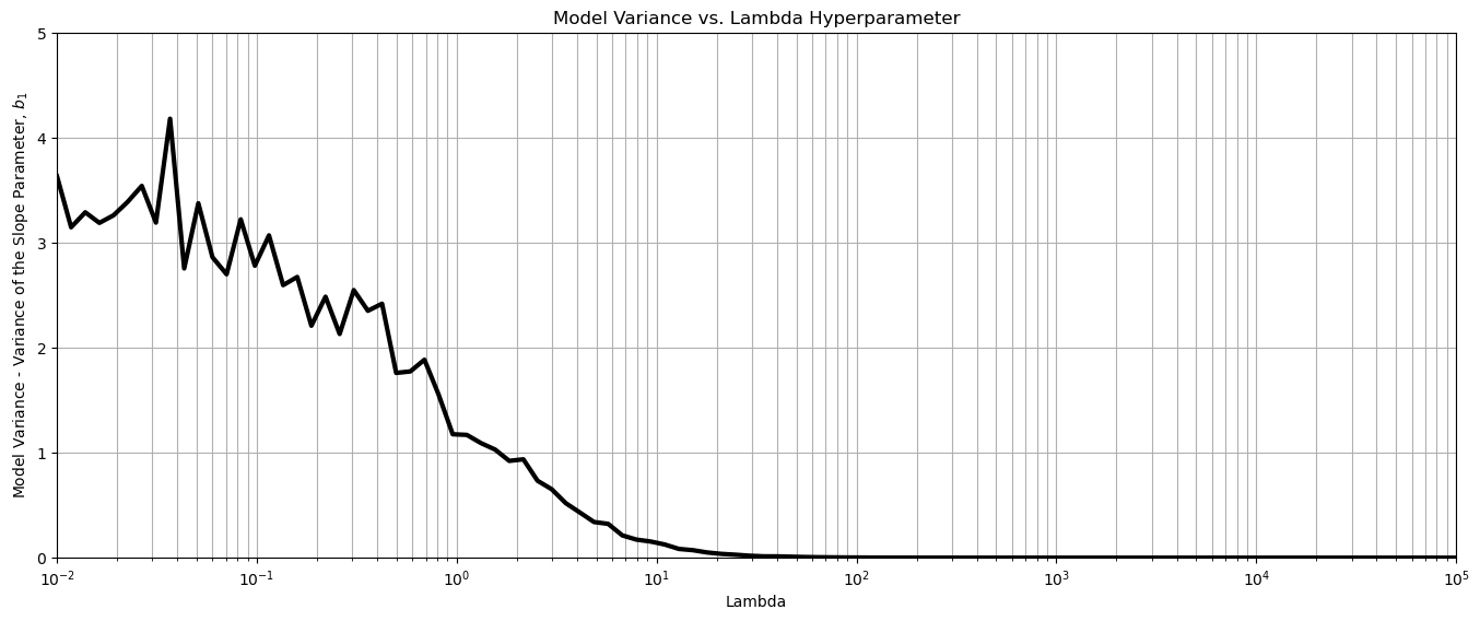
The result is as expected, with increase in \(\lambda\) hyperparameter the sensitivity of the model to the training data is decreased.
k-fold Cross Validation#
It would be useful to conduct a complete k-fold validation to evaluate the testing error vs. the hyperparameter lambda for model tuning.
the following code is provided to do this
once again, with a single predictor feature we must reshape to a 2D array
We loop over 100 \(\lambda\) values from 0.01 to 100,000,
get the negative mean square error for each of the 4 k-folds
then we take the average and apply the absolute value
Why work with negative mean square error? Simple, to use the functionality in scikit-learn that optimizes by maximization and for consistency with other scores like \(r^2\) where larger values are better.
I find negative MSE confusing, so for plotting I use the absolute value to convert the values to strictly positive.
score = []                                                    # code modified from StackOverFlow by Dimosthenis

nlambda = 100
lambda_mat = np.logspace(-2,5,nlambda)
for ilam in range(0,nlambda):
    ridge_reg = Ridge(alpha=lambda_mat[ilam])
    scores = cross_val_score(estimator=ridge_reg, X= df['Density'].values.reshape(-1, 1), y=df['Porosity'].values, cv=10, n_jobs=4, scoring = "neg_mean_squared_error") # Perform 10-fold cross validation
    score.append(abs(scores.mean()))

plt.subplot(111)
plt.plot(lambda_mat, score,  color='black', linewidth = 3, label = 'Test MSA',zorder=10)
plt.title('Ridge Regression Test Mean Square Error vs. Lambda Hyperparameter'); plt.xlabel('Lambda'); plt.ylabel('Test Mean Square Error')
plt.xlim(1.0e-2,1.0e5); plt.ylim(0.001,20.0); plt.xscale('log')
plt.vlines(0.5,0,20,color='red',lw=2); plt.vlines(1000,0,20,color='red',lw=2,zorder=10)
plt.annotate('Linear Regression',[0.4,12.5],rotation=90.0,color='red',zorder=10)
plt.annotate('Mean',[1100,14.5],rotation=90.0,color='red',zorder=10)
plt.fill_between([0.01,0.5],[0,0],[20,20],color='grey',alpha=0.3,zorder=1)
plt.fill_between([1000,100000],[0,0],[20,20],color='grey',alpha=0.3,zorder=1)
plt.grid(which='both')
plt.subplots_adjust(left=0.0, bottom=0.0, right=2.0, top=1.0, wspace=0.2, hspace=0.2); plt.show()
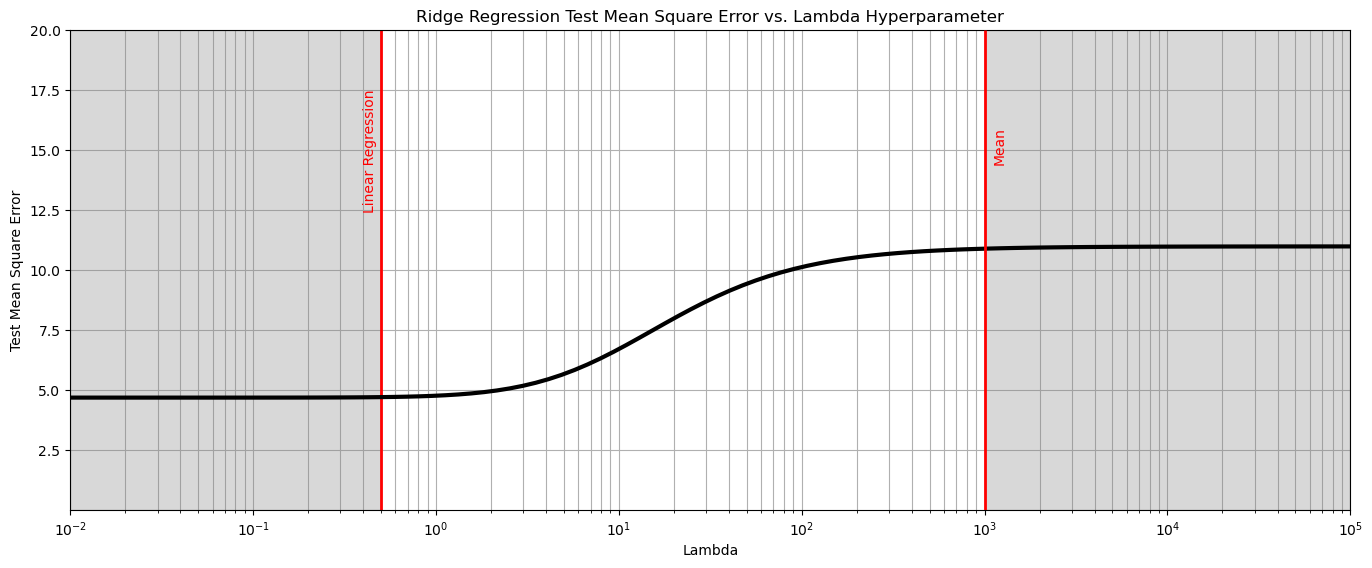
From the above we observe 3 phases,
left - the test MSE levels out at a minimum, the model has converged on linear regression.
right - the test MSE levels out at a maximum, the model has converged on the predictor feature mean, i.e., model parameter slope is 0.0.
center - transitional between both cases
In this case we see that the linear regression model (\(\lambda = 0.0\)) is the best model! If ridge regression is the optimum model the test mean square error would minimize between linear regression and mean.
this commonly occurs for datasets with issues with noise, data paucity and high dimensionality.
our model is the same as linear regression.
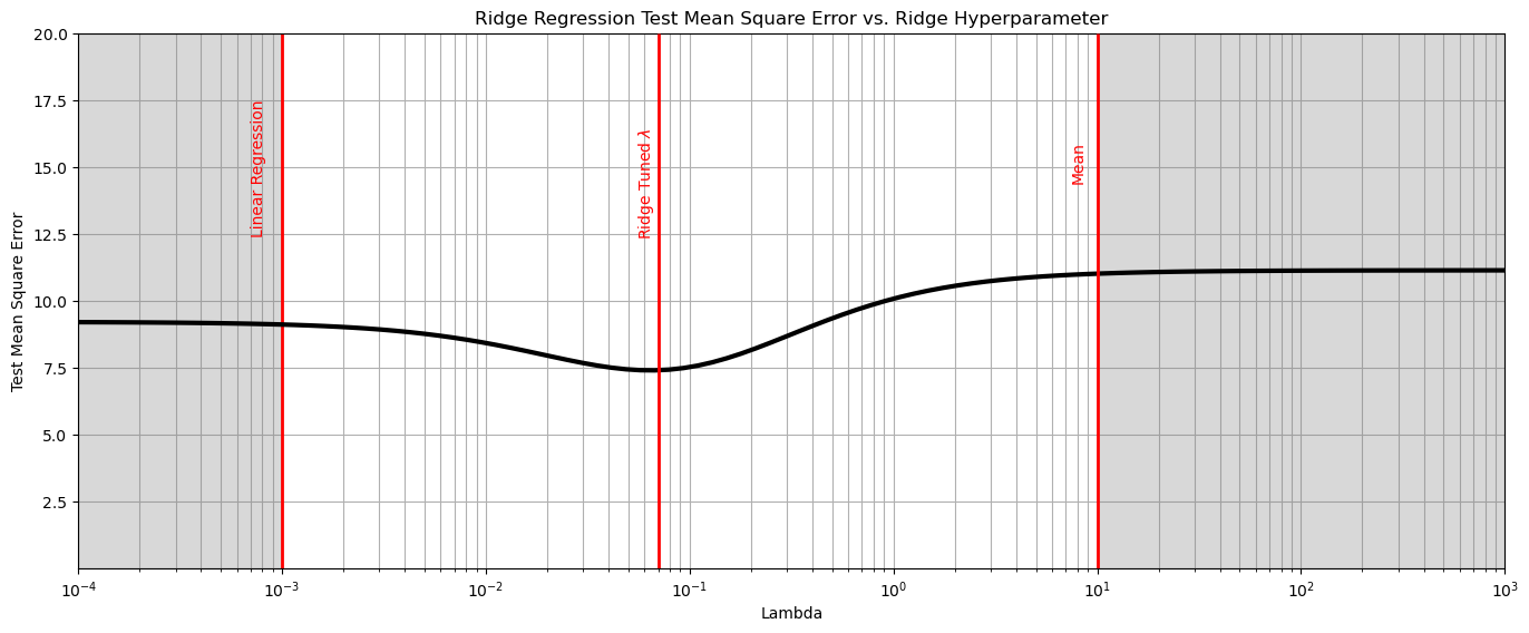
could we create a situation where the best model is not linear regression? I.e., were regularization is helpful?
yes, we can. Let’s remove most the samples to create data paucity and add a lot of noise!
Admittedly, I iterated the random seeds for the sample and noise to get this result.
few data (low \(n\)) and high dimensionality (high \(m\)) will generally result in LASSO outperforming linear regression
df_sample = df.copy(deep=True).sample(n=10,random_state=11)
noise_stdev = 3.0
np.random.seed(seed=15)
df_sample['Porosity'] = df_sample['Porosity'] + np.random.normal(0.0, noise_stdev, size=len(df_sample))

score = []                                                    # code modified from StackOverFlow by Dimosthenis

nlambda = 100
lambda_mat = np.logspace(-4,3,nlambda)
for ilam in range(0,nlambda):
    ridge_reg = Ridge(alpha=lambda_mat[ilam])
    scores = cross_val_score(estimator=ridge_reg, X= df_sample['Density'].values.reshape(-1, 1),
                             y=df_sample['Porosity'].values, cv=2, n_jobs=4, scoring = "neg_mean_squared_error") # Perform 10-fold cross validation
    score.append(abs(scores.mean()))

plt.subplot(111)
plt.plot(lambda_mat, score,  color='black', linewidth = 3, label = 'Test MSA',zorder=10)
plt.title('Ridge Regression Test Mean Square Error vs. Ridge Hyperparameter'); plt.xlabel('Lambda'); plt.ylabel('Test Mean Square Error')
plt.xlim(1.0e-4,1.0e3); plt.ylim(0.001,20.0);
plt.xscale('log')
plt.vlines(0.001,0,20,color='red',lw=2); plt.vlines(10,0,20,color='red',lw=2,zorder=10);
plt.vlines(0.07,0,20,color='red',lw=2,zorder=10);
plt.annotate('Linear Regression',[0.0007,12.5],rotation=90.0,color='red',zorder=10)
plt.annotate(r'Ridge Tuned $\lambda$',[0.055,12.5],rotation=90.0,color='red',zorder=10)
plt.annotate('Mean',[7.4,14.5],rotation=90.0,color='red',zorder=10)
plt.fill_between([0.0001,0.001],[0,0],[20,20],color='grey',alpha=0.3,zorder=1)
plt.fill_between([10,100000],[0,0],[20,20],color='grey',alpha=0.3,zorder=1)
plt.grid(which='both')
plt.subplots_adjust(left=0.0, bottom=0.0, right=2.0, top=1.0, wspace=0.2, hspace=0.2); plt.show()
About the Author#

Michael Pyrcz is a professor in the Cockrell School of Engineering, and the Jackson School of Geosciences, at The University of Texas at Austin, where he researches and teaches subsurface, spatial data analytics, geostatistics, and machine learning. Michael is also,
the principal investigator of the Energy Analytics freshmen research initiative and a core faculty in the Machine Learn Laboratory in the College of Natural Sciences, The University of Texas at Austin
an associate editor for Computers and Geosciences, and a board member for Mathematical Geosciences, the International Association for Mathematical Geosciences.
Michael has written over 70 peer-reviewed publications, a Python package for spatial data analytics, co-authored a textbook on spatial data analytics, Geostatistical Reservoir Modeling and author of two recently released e-books, Applied Geostatistics in Python: a Hands-on Guide with GeostatsPy and Applied Machine Learning in Python: a Hands-on Guide with Code.
All of Michael’s university lectures are available on his YouTube Channel with links to 100s of Python interactive dashboards and well-documented workflows in over 40 repositories on his GitHub account, to support any interested students and working professionals with evergreen content. To find out more about Michael’s work and shared educational resources visit his Website.
Want to Work Together?#
I hope this content is helpful to those that want to learn more about subsurface modeling, data analytics and machine learning. Students and working professionals are welcome to participate.
Want to invite me to visit your company for training, mentoring, project review, workflow design and / or consulting? I’d be happy to drop by and work with you!
Interested in partnering, supporting my graduate student research or my Subsurface Data Analytics and Machine Learning consortium (co-PI is Professor John Foster)? My research combines data analytics, stochastic modeling and machine learning theory with practice to develop novel methods and workflows to add value. We are solving challenging subsurface problems!
I can be reached at mpyrcz@austin.utexas.edu.
I’m always happy to discuss,
Michael
Michael Pyrcz, Ph.D., P.Eng. Professor, Cockrell School of Engineering and The Jackson School of Geosciences, The University of Texas at Austin
More Resources Available at: Twitter | GitHub | Website | GoogleScholar | Geostatistics Book | YouTube | Applied Geostats in Python e-book | Applied Machine Learning in Python e-book | LinkedIn
Comments#
This was a basic treatment of ridge regression. Much more could be done and discussed, I have many more resources. Check out my shared resource inventory and the YouTube lecture links at the start of this chapter with resource links in the videos’ descriptions.
I hope this is helpful,
Michael