Machine Learning Concepts

Machine Learning Concepts#

Michael J. Pyrcz, Professor, The University of Texas at Austin

Chapter of e-book “Applied Machine Learning in Python: a Hands-on Guide with Code”.

Cite this e-Book as:

Pyrcz, M.J., 2024, Applied Machine Learning in Python: A Hands-on Guide with Code [e-book]. Zenodo. doi:10.5281/zenodo.15169138

The workflows in this book and more are available here:

Cite the MachineLearningDemos GitHub Repository as:

Pyrcz, M.J., 2024, MachineLearningDemos: Python Machine Learning Demonstration Workflows Repository (0.0.3) [Software]. Zenodo. DOI: 10.5281/zenodo.13835312. GitHub repository: GeostatsGuy/MachineLearningDemos

By Michael J. Pyrcz
© Copyright 2024.

This chapter is a summary of Machine Learning Concepts including essential concepts:

Statistics and Data Analytics
Inferential Machine Learning
Predictive Machine Learning
Machine Learning Model Training and Tuning
Machine Learning Model Overfit

YouTube Lecture: check out my lecture on Introduction to Machine Learning. For your convenience here’s a summary of salient points.

Motivation for Machine Learning Concepts#

You could just open up a Jupyter notebook in Python and start building machine learning models.

the scikit-learn docs are quite good and for every machine learning function there is a short code example that you could copy and paste to repeat their work.
also, you could Google a question about using a specific machine learning algorithm in Python and the top results will include StackOverflow questions and responses, it is truly amazing how much experienced coders are willing to give back and share their knowledge. We truly have an amazing scientific community with the spirit of knowledge sharing and open-source development. Respect.
of course, you could learn a lot about machine learning from a machine learning large language model (LLM) like ChatGPT. Not only will ChatGPT answer your questions, but it will also provide codes and help you debug them when you tell it what went wrong.

One way of the other and you received and added this code to you data science workflow,

n_neighbours = 10; weights = "distance"; p = 2
neigh = KNeighborsRegressor(n_neighbors=n_neighbours,weights = weights,p = p).fit(X_train,y_train) 

et voilà (note I’m Canadian, so I use some French phrases), you have a trained predictive machine learning model that could be applied to make predictions for new cases.

But, is this a good model?
How good is it?
Could it be better?

Without knowledge about basic machine learning concepts we can’t answer these questions and build the best possible models. In general, I’m not an advocate for black box modeling, because it is:

likely to lead to mistakes that may be difficult to detect and correct
incompatible with the expectations for competent practice for professional engineers. I gave a talk on Applying Machine Learning as a Compentent Engineer or Geoscientist

To help out this chapter provides you with the basic knowledge to answer these questions and to make better, more reliable machine learning models. Let’s start building this essential foundation with some definitions.

Big Data#

Everyone hears that machine learning needs a lot of data. In fact, so much data that it is called “big data”, but how do you know if you are working with big data?

the criteria for big data are these ‘V’s

If you answer “yes” for at least some of these criteria, then you are working with big data,

Volume: many data samples, difficult to handle and visualize
Velocity: high rate collection, continuous relative to decision making cycles
Variety: data form various sources, with various types and scales
Variability: data acquisition changes during the project
Veracity: data has various levels of accuracy

In my experience, most subsurface engineers and geoscientists answer “yes” to all of these ‘v’ criteria.

so I proudly say that we in the subsurface have been big data long before the tech sector learned about big data

In fact, I often state that we in the subsurface resource industries are the original data scientists.

I’m getting ahead of myself, more on this in a bit. Don’t worry if I get carried away in hubris, rest assured this e-book is written for anyone interested to learn about machine learning.
you can skip the short sections on subsurface data science or read along if interested.

Now that we know big data, let’s talk about the big data related topics, statistics, geostatistics and data analytics.

Statistics, Geostatistics and Data Analytics#

Statistics is the practice of,

collecting data
organizing data
interpreting data
drawing conclusions from data
making decisions with data

It is all about moving from data to decision.

The importance of decision making in statistics.

If your work does not impact the decision, you do not add value!

If you look up the definition of data analytics, you will find criteria that include, statistical analysis, and data visualization to support decision making.

I call it, data analytics and statistics are the same thing.

Now we can append, geostatistics as a branch of applied statistics that accounts for,

the spatial (geological) context
the spatial relationships
volumetric support
uncertainty

Remember all those statistics classes with the assumption of i.i.d., independent, identically distributed.

spatial phenomenon are not i.i.d., so we developed a unique branch of statistics to address this
by our assumption above (statistics is data analytics), we can state that geostatistics is the same as spatial data analytics

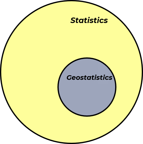
Now, let’s use a Venn diagram to visualize statistics / data analytics and geostatistics / spatial data analytics,

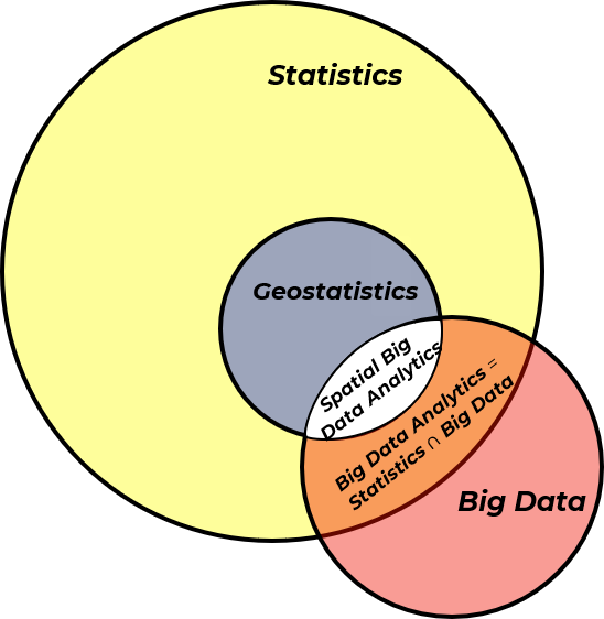
Venn diagram for statistics and geostatistics.

and we can add our previously discussed big data to our Venn diagram resulting in big data analytics and spatial big data analytics.

Venn diagram for statistics and geostatistics with big data added.

Scientific Paradigms and the Fourth Paradigm#

If no one else has said this to you, let me have the honor of saying,

Welcome

to the fourth paradigm of scientific discovery, data-driven scientific discovery or we can just call it data science.

The paradigms of scientific discovery are distinct approaches for humanity to apply science to expand human knowledge, discover and develop new technologies that impact society. These paradigms include,

First Paradigm - logical reasoning with physical experiment and observation
Second Paradigm - theory-driven, where mathematical models and laws are used to explain and predict natural phenomena
Third Paradigm - computer-based numerical simulations and models to study complex systems that are too difficult or impossible to solve analytically or test experimentally
Fourth Paradigm - analysis of massive datasets with tools such as data analytics, machine learning, cloud computing and AI, patterns in the data guide insights.

Here’s all of the four paradigms with dates for important developments with each,

1st Paradigm Empirical Science	2nd Paradigm Theoretical Science	3rd Paradigm Computational Science	4th Paradigm Data Science
Logic and Experiments	Theory and Models	Numerical Simulation	Learning from Data
\(\approx\) 600 BC Thales of Miletus predicted a solar ecplipse	\(\approx\) 300 BC Euclid - Elements	1946 von Neumann weather simulation	1990s Human Genome Project
\(\approx\) 400 BC Hippocrates natural causes for diseases	\(\approx\) 150 AD Ptolemy planetary motion model	1952 Fermi simulated nonlinear systems	2008 Large Hadron Collider
430 BC Empedocles proved air has substance	1011 AD al-Haytham Book of Optics	1957 Lorenz demonstrates chaos	2009 Hey et al. Data-Intensive Book
230 BC Eratosthenes measures Earth’s diameter	1687 AD Newton Principia	1980s Mandelbrot simulating fractals	2015 AlphaGo beats a professional Go player

Of course, we can argue about the boundaries between the paradigms for scientific discovery, i.e., when did a specific paradigm begin? For example, consider these examples of the application of the first paradigm that push the start of the first paradigm deep into antiquity!

Field	Example	Approx. Date	Why It Fits 1st Paradigm
Agriculture	Irrigation systems using canals, gates, and timing	\(\approx\) 3000 BC	Empirical understanding of water flow, soil, and seasonal timing
Astronomy	Babylonian star charts; lunar calendars	\(\approx\) 1800 BC	Systematic observations for predicting celestial events
Engineering	The wheel (transport, pottery)	\(\approx\) 3500 BC	Developed through trial-and-error and practical refinement
Medicine	Herbal remedies, surgical procedures	\(\approx\) 2000 BC	Based on observation and accumulated case knowledge
Mathematics	Base-60 system; geometric calculation tablets	\(\approx\) 2000 BC	Used for land division, architecture, and astronomy; empirically tested

certainly the Mesopotamians (4000 BC - 3500 BC) applied the first paradigm with their experiments that supported the development of the wheel, plow, chariot, weaving loom, and irrigation. Aside, I wanted to give a shout out to the ancient peoples, because I’m quite fascinated by the development of human societies and their technologies over time.

On the other side, we can trace the development of fourth paradigm approaches, for example the artificial neural networks to McColloch and Pitts in 1943 and consider these early examples of learning by distilling patterns from large datasets,

Year	Field	Example / Person	Why It Fits 4th Paradigm Traits
\(\approx\)100 AD	Astronomy	Ptolemy’s star catalog	Massive empirical data used to predict celestial motion
1086	Economics	Domesday Book (England)	Large-scale data census for administrative, economic decisions
1700s	Natural history	Carl Linnaeus – taxonomy	Classification of species based on observable traits; data-first approach
1801	Statistics	Adolphe Quetelet – social physics	Used statistics to analyze human behavior from large datasets
1830s	Astronomy	John Herschel’s sky surveys	Cataloged thousands of stars and nebulae; data-driven sky classification
1859	Biology	Darwin – Origin of Species	Synthesized global species data to uncover evolutionary patterns
1890	Public health	Florence Nightingale	Used mortality data visualization to influence hospital reform
1890	Census, Computing	Hollerith punch cards (U.S. Census)	First automated analysis of large datasets; mechanical data processing
1910s–30s	Genetics	Morgan lab – Drosophila studies	Mapped gene traits from thousands of fruit fly crosses
1920s	Economics	Kondratiev, Kuznets	Identified economic patterns using historical data series
1937	Ecology	Arthur Tansley – ecosystem concept	Integrated large-scale field data into systemic ecological frameworks

Finally, the adoption of a new scientific paradigm represents a significant societal shift that unfolds unevenly across the globe. While I aim to summarize the chronology, it’s important to acknowledge its complexity.

Foundations and Enablers of the Fourth Scientific Paradigm#

What caused the fourth paradigm to start some time between 1943 and 2009? Is it the development of new math?

the foundational mathematics behind data-driven models has been available for decades and even centuries. Consider the following examples of mathematical and statistical developments that underpin modern data science,

Technique	Key Contributor(s)	Date / Publication
Calculus	Isaac Newton, Gottfried Wilhelm Leibniz	Newton: Methods of Fluxions (1671, pub. 1736); Leibniz: Nova Methodus (1684)
Bayesian Probability	Reverend Thomas Bayes	An Essay Towards Solving a Problem in the Doctrine of Chances (posthumous, 1763)
Linear Regression	Marie Legendre	Formalized in 1805
Discriminant Analysis	Ronald Fisher	The Use of Multiple Measurements in Taxonomic Problems (1939)
Monte Carlo Simulation	Stanislaw Ulam, John von Neumann	Developed in early 1940s during the Manhattan Project

Upon reflection, one might ask: why didn’t the fourth scientific paradigm emerge earlier—say, in the 1800s or even before the 1940s? What changed? The answer lies in the fact that several key developments were still needed to create the fertile ground for data science to take root.

Specifically:

the availability of inexpensive, accessible computing power
the emergence of massive, high-volume datasets (big data)

Let’s explore each of these in more detail.

Cheap and Available Compute#

Learning from big data is not feasible without affordable and widely available computing and storage resources. Consider the following computational advancements that paved the way for the emergence of the fourth scientific paradigm,

Year	Milestone	Description
1837	Babbage’s Analytical Engine	First design of a mechanical computer with concepts like memory and control flow (not built).
1941–45	Zuse’s Z3, ENIAC	First programmable digital computers; rewired plugboards, limited memory, slow and unreliable.
1947	Transistor Invented	Replaced vacuum tubes; enabled faster, smaller, more reliable second-gen computers (e.g., IBM 7090).
1960s	Integrated Circuits	Multiple transistors on a single chip; led to third-generation computers.
1971	Microprocessor Developed	Integrated CPU on a chip; enabled personal computers like Apple II (1977) and IBM PC (1981).

Yes, when I was in grade 1 of my elementary school education we had the first computers in classrooms (Apple IIe), and it amazed all of us with the monochrome (orange and black pixels) monitor, 5 1/4 inch floppy disk loaded programs (there was no hard drive) and the beeps and clicks from the computer (no dedicated sound chip)!

We live in a society with more compute power in our pockets, i.e., our cell phones, than used to send the first astronauts to the moon and a SETI screen saver that uses home computers’ idle time to search for extraterrestrial life!

SETI@home - search for extraterrestrial intelligence. Note the @home component is now in hibernation while the team continuous the analysis the data.

Also check out these ways to put your computer’s idle time to good use,

Folding@home - simulate protein dynamics, including the process of protein folding and the movements of proteins to develop therapeutics for treating disease.
Einstein@home - search for weak astrophysical signals from spinning neutron stars, with big data from the LIGO gravitational-wave detectors, the MeerKAT radio telescope, the Fermi gamma-ray satellite, and the archival data from the Arecibo radio telescope.

Now we are surrounded by cheap and reliable compute that our grandparents (and perhaps even our parents) could scarcely have imagined.

As you will learn in this e-book, machine learning methods requires a lot of compute, because training most of these methods relies on,

numerous iterations
matrix or parallel computations
bootstrapping techniques
stochastic gradient descent
extensive model tuning, which may involve training many versions in nested loops

Affordable and accessible computing is a fundamental prerequisite for the fourth scientific paradigm.

the development of data science has been largely driven by crowd-sourced and open-source contributions—efforts that rely on widespread access to computing power

In the era of Babbage’s Analytical Engine or the ENIAC, data science at scale would have been simply impossible.

Availability of Big Data#

With small data, we often rely on external sources of knowledge such as:

Physics
Engineering and geoscience principles

These models are then calibrated using the limited available observations—a common approach in the second and third scientific paradigms.

In contrast, big data allows us to learn the full range of behaviors of natural systems directly from the data itself. In fact, big data often reveals the limitations of second and third paradigm models, exposing missing complexities in our traditional solutions.

Therefore, big data is essential to:

provide sufficient sampling to support the data-driven fourth paradigm

It may even challenge the exclusive reliance on second and third paradigm models, as the complexity of large datasets uncovers the boundaries of our existing theoretical frameworks.

Today, big data is everywhere! Consider all the open-source and publically available data online. Here’s some great examples,

Resource	Description	Link
Google Earth (Timelapse)	Satellite imagery (not highest res, but useful for land use, geomorphology, and surface evolution studies). Used by research teams.	Google Earth
USGS River Gage Data	Public streamflow and hydrology data; useful for analysis and recreational planning (e.g., paddling).	USGS NWIS
Government Databases	Includes U.S. Census and oil & gas production statistics. Open for public and research use.	U.S. Census, Texas Oil & Gas Data
NASA Moon Trek	High-res lunar surface imagery from LRO, SELENE, and Clementine; interactive visualization and downloads.	Moon Trek
Landsat Satellite Archive	50+ years of medium-resolution Earth observation data (since 1972); invaluable for land cover change.	USGS EarthExplorer
Copernicus Open Access Hub	European Space Agency’s Sentinel satellite data (e.g., radar, multispectral imagery).	Copernicus Hub
Global Biodiversity Information Facility (GBIF)	Open biodiversity data: species distributions, observations, and ecological records from around the world.	GBIF
National Oceanic and Atmospheric Administration (NOAA)	Huge archive of weather, ocean, and climate data, including radar, reanalysis, and forecasts.	NOAA Data
World Bank Open Data	Economic, development, demographic, and environmental indicators for all countries.	World Bank Data
Our World in Data	Curated global datasets on health, population, energy, CO₂, education, and more.	Our World in Data
OpenStreetMap (OSM)	Crowdsourced global geospatial data including roads, buildings, and land use.	OpenStreetMap
Google Dataset Search	Meta-search engine indexing datasets across disciplines and repositories.	Dataset Search

While open data is rapidly expanding, proprietary data is also growing quickly across many industries, driven by the adoption of smart, connected systems with advanced monitoring and control.

The result of all of this is a massive explosion of data, supported by faster, more affordable computing, processing, and storage. We are now immersed in a sea of data that previous generations could never have imagined.

Note, we could also talk about improved algorithms and hardware architectures optimized for data science, but I’ll leave that out of scope for this e-book.

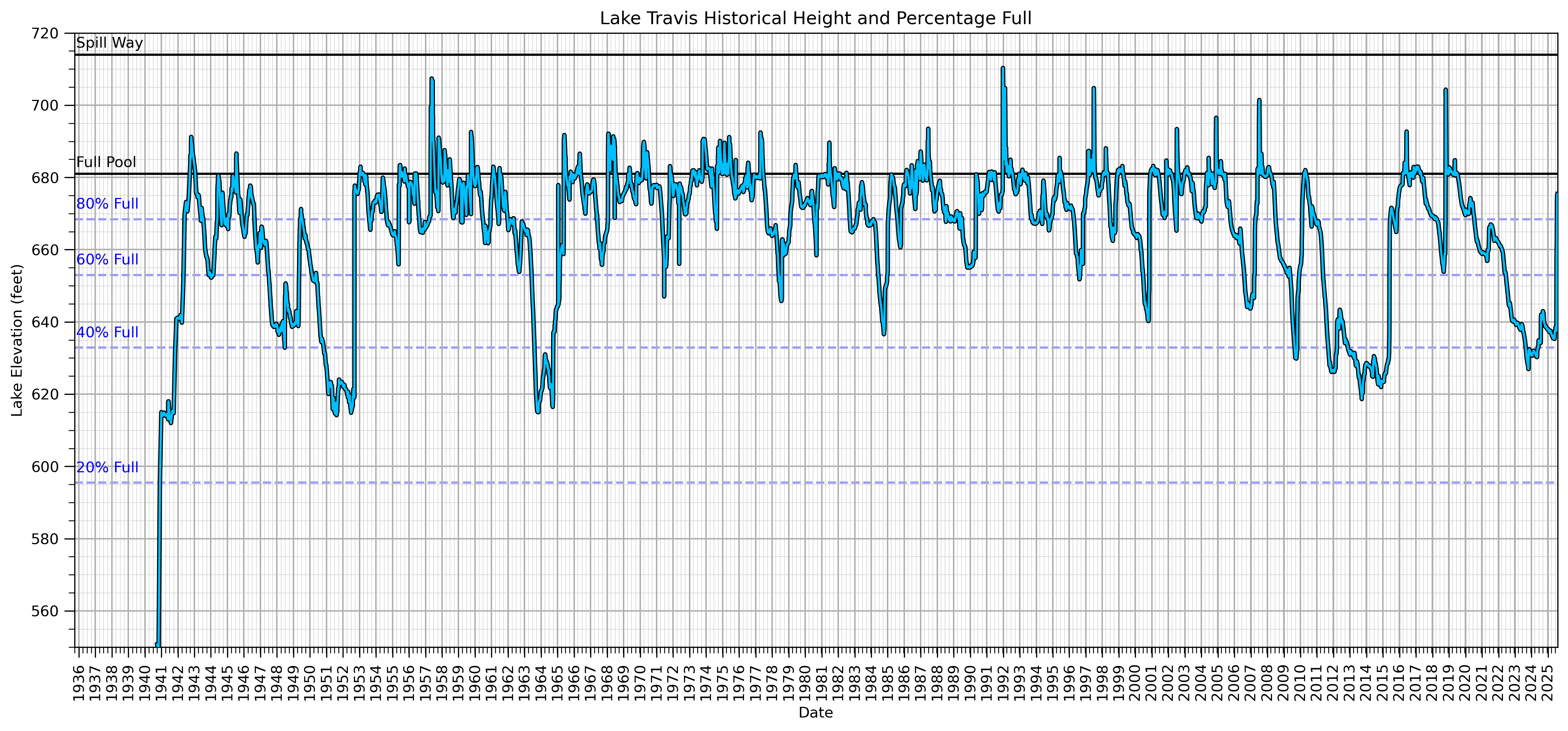
Here’s a local example of freely available big data. I downloaded the daily water level of our local Lake Travis from Water Data for Texas. Note the data is collected and provided by Lower Colorado Water Authority LRCA.

I made a plot of the daily plot and added useful information such as,

water height - in feet above mean sea level
percentage full - the ratio of the current volume of water stored in a reservoir to its total storage capacity, expressed as a percentage, accounting for the shape of the reservoir
max pool - maximum conservation pool, the top of the reservoir used for water supply, irrigation, hydropower and recreation and not including flood storage.

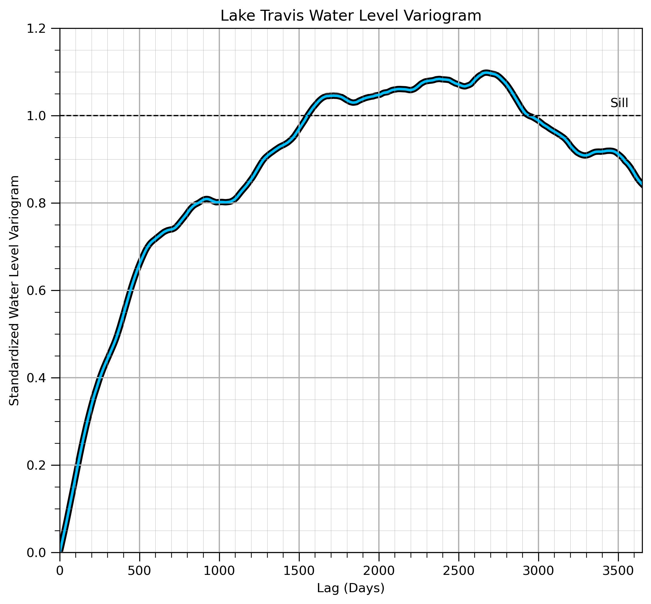
Historical Lake Austin daily water level and percentage full.

And before you even ask - yes! I did calculate the semivariogram of water level and I was surprised that there was no significant nuggest effect.

Historical Lake Austin daily water level variogram.

To become a good data scientists!

Find and play with data!

All of these developments have provided the fertile ground for the seeds of data science to impact all sectors or our economy and society.

Data Science and Subsurface Resources#

Spoiler alert, I’m going to boast a bit in the section. I often hear students say,

“I can’t believe this data science course is in the Hildebrand Department of Petroleum and Geosystems Engineering!”
“Why are you teaching machine learning in Department of Earth and Planetary Sciences?”

Once again, my response is,

We in the subsurface are the original data scientists!

We have been big data long before tech learned about big data!

This may sound a bit arrogant, but let me back this statement up with this timeline,

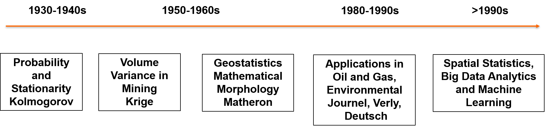
Timeline of data science development from the perspective of subsurface engineering and geoscience.

Shortly after Kolmogorov developed the fundamental probability axioms, Danie Krige developed a set of statistical, spatial, i.e., data-driven tools for making estimates in space while accounting for spatial continuity and scale. These tools were formalized with theory developed by Professor Matheron during the 1960s in a new science called geostatistics. Over the 1970s - 1990s the geostatistical methods and applications expanded from mining to address oil and gas, environmental, agriculture, fisheries, etc. with many important open source developments.

Why was subsurface engineering and geoscience earlier in the development of data science?

because, necessity is the mother of invention! Complicated, heterogeneous, sparsely sampled, vast systems with complicated physics and high value decisions drove us to data-driven methods.

There are many other engineering fields that had little motivation to develop and apply data science due to,

homogeneous phenomenon that does not have significant spatial heterogeneity, continuity, nor uncertainty - with few samples the phenomenon is sufficiently understood, for example, sheet aluminum used for aircraft or cement used in structures
exhaustive sampling of the population relative to the modeling purpose and do not need an estimation model with uncertainty - the phenomenon’s properties are known and the performance can be simulated in a finite element model, for example, radiographic testing for cracks in a machine housing
have well understood physics and can model the entire system with second and third paradigm phenomenon - the (coupled) physics is known and can be modeled, for example, the Boeing 777 was the first commerical airliner designed entirely using computed-aided design (CAD)

Compare this to the typical context of subsurface engineering and geoscience, where data challenges are both unique and substantial:

Sparsely sampled datasets – we often sample only a minuscule fraction—sometimes as little as one hundred-billionth—of the subsurface volume of interest. This leads to significant uncertainty and a heavy reliance on statistical and data-driven models.
Massively multivariate datasets – integrating diverse data types (e.g., seismic, well logs, core data) poses a major challenge, requiring robust multivariate statistical and machine learning techniques.
Complex, heterogeneous earth systems – subsurface geology is highly variable and location-dependent. These open systems often behave unpredictably, demanding flexible and adaptive modeling approaches.
High-stakes, high-cost decisions – The need to support critical, high-value decisions drives innovation in methods, workflows, and the adoption of advanced analytics.

As a result, many of us in subsurface engineering and geoscience have a lot of experience learning, applying, and teaching data science to better understand and manage these complexities.

Machine Learning#

Now we are ready to define machine learning, a Wikipedia artical on Machine Learning can be summarized and broken down as follows, machine learning has these aspects,

toolbox - a collections of algorithms and mathematical models used by computer systems
learning - that improve their performance progressively on a specific task
training data - by learning patterns from sample data
general - to make predictions or decisions without being explicitly programmed for the specific task

Let’s highlight some key ideas:

machine learning is a numerical toolbox, a broad set of algorithms designed to adapt to different problems (toolbox)
these algorithms improve by learning from or fitting to training data (learning from training data)
a single algorithm can often be trained and applied across many different domains (generalization)

An especially important point, often overlooked is found near the end of the article:

This underscores that machine learning is most valuable when traditional rule-based programming becomes too complex, impractical, or infeasible, often due to the scale or variability of the task.

In other words, if the underlying theory is well understood, be it engineering principles, geoscience fundamentals, physics, chemical reactions, or mechanical systems, then use that knowledge first.

don’t rely on data science as a replacement for foundational understanding of science and engineering (Paraphrased from personal communication with Professor Carlos Torres-Verdin, 2024)

Machine Learning Prerequisite Definitions#

To understand machine learning and in general, data science we need to first differentiate between the population and the sample.

Population#

The population is all possible information of our spatial phenomenon of interest. Exhaustive, finite list of feature of interest over area of interest at the resolution of the data. For example,

exhaustive set of porosity at every location within a gas reservoir at the scale of a core sample, i.e., imagine the entire reservoir drilled, extracted and analyzed core by core!
for every tree in a forest the species, diameter at breast height (DBH), crown diameter, age, tree health status, wood volume and location, i.e., perfectly knowledge of our forest!

Generally the entire population is not accessible due to,

technology limits - sampling methods that provide improved coverage generally have reduced resolution and accuracy
practicallity - removing too much reservoir will impact geomechanical stability
cost - wells cost 10s - 100s of millions of dollars each

Sample#

The limited set of values, at specific locations that have been measured. For example,

limited set of porosity values measured from extracted core sample and callibrated from well-logs within a reservoir
1,000 randomly selected trees over an management unit, with species, diameter at breast height (DBH), crown diameter, age, tree health status, wood volume and location

There is so much that I could mention about sampling! For example,

methods for representative sample selection
impact of sample frequency or coverage on uncertainty and required levels of sampling
methods to debias biased spatial samples (see Declustering to Debias Data from my Applied Geostatistics in Python e-book

For brevity I will not cover these topics here, but let’s now dive into,

What are we measuring from our population in our samples?

Each distinct type of measure is called a variable or feature.

Variable or Feature#

In any scientific or engineering study, a property that is measured or observed is typically referred to as a variable.

however, in data science and machine learning, we use the term feature almost exclusively.

While the terminology differs, the concept is the same: both refer to quantitative or categorical information about an object or system.

To illustrate what constitutes a feature, consider the following examples drawn from real-world geoscience, oil adn gas, and mining contexts,

porosity measured from 1.5 inch diameter, 2 inch long core plugs extracted from the Miocene-aged Tahiti field in the Gulf of Mexico
permeability modeled from porosity (neutron density well log) and rock facies (interpreted fraction of shale logs) at 0.5 foot resolution along the well bore in the Late Devonian Leduc formation in the Western Canadian Sedimentary Basin.
blast hole cuttings nickel grade aggregated over 8 inch diameter 10 meter blast holes at Voisey’s Bay Mine, Proterozoic gneissic complex.

Did you see what I did?

I specified what was measured, how it was measured, and over what scale was it measured.

This is important because,

how the measurement is made? - changes the feature’s veracity (level of certainty in the measure) and different methods actually may change the shift the feature’s values so we may need to reconcile multiple measurement methods of the same feature.
what is the scale of the measurement? - is very important due to volume-variance effect, with increasing support volume, sample scale, the variance reduces due to volumetric averaging resulting in regression to the mean. I have a chapter on volume-variance in my Applied Geostatistics in Python e-book for those interested in more details.

Additionally, our subsurface measurements often requires significant analysis, interpretation, etc.

we don’t just hold a tool up to the rock and get the number
we have a “thick layer” of engineering and geoscience interpretation to map from measurement to a useable feature.

Consider this carbonate thin section from Bureau of Economic Geology, The University of Texas at Austin from geoscience course by F. Jerry Lucia.

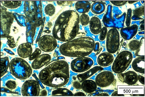
Carbonate thin section image (from this link by F. Jerry Lucia).

Note: the blue dye in core samples visually indicates void space—the pores in the rock. But is the porosity feature simply the blue area divided by the total area of the sample?

that would give us total porosity, which is the ratio of total void volume to bulk volume
however, not all pore space contributes to fluid flow. Some pores are isolated or poorly connected, especially in low-permeability rocks

To estimate the porosity that actually matters for flow, we need to interpret connectivity. This gives us effective porosity, a more useful feature for modeling fluid transport, permeability, and reservoir performance.

so even porosity, often seen as a “simple” feature that’s observable in well logs and suitable for linear averaging, doesn’t escape an essential interpretation step. Estimating effective porosity involves assumptions, thresholds, or models about pore geometry and connectivity.

This is a critical reminder, our features generally require interpretation, even when they appear directly measurable. Measurement scale, observation method, and intended use all influence how we define and derive a useful feature for our data science models.

Predictor and Response Features#

To understand the difference between predictor and response features let’s look at the most concise expression of a machine learning model.

The fundamental predictive machine learning model that maps from predictor to response features.

the predictors (or independent) features (or variables) the model inputs, i.e., the \(X_1,\ldots,X_m\)
response (or dependent) feature(s) (or variable(s)) are the model output, \(y\),

and there is an error term, \(\epsilon\).

Machine Learning is all about estimating such models, \(\hat{𝑓}\), for two purposes, inference or prediction.

Inference#

Before we can make reliable predictions, we must first perform inference—that is, we must learn about the underlying system from a limited sample in order to model the broader population. Inference is the process of building an understanding of the system, denoted as \(\hat{f}\), based on observed data.

Through inference, we seek to answer questions like:

What are the relationships between features?
Which features are most important?
Are there complicated or nonlinear interactions between features?

These insights are prerequisites for making any predictions, because they form the foundation of the model that will eventually be used for forecasting, classification, or decision-making.

For example, imagine I walk into a room, pull a coin from my pocket, and flip it 10 times, observing 3 heads and 7 tails. Then I ask, “Is this a fair coin?”.

This is a classic inferential problem.

you’re using a limited sample (the 10 flips) to make an inference about the population—in this case, the probability distribution governing the coin
and here’s the key twist: in this example, the coin itself is the population!

You’re not just summarizing the sample, you’re trying to learn something general about the system that generated the sample.

Prediction#

Once we’ve completed inference—learning from a sample to build a model of the underlying population—we’re ready to use that model for prediction. Prediction is the process of applying what we’ve learned to estimate the outcomes of new or future observations.

in short, inference goes from sample to the population, while prediction goes from population model to the new sample
the goal of prediction is to produce the most accurate estimates of unknown or future outcomes

Let’s return to our earlier coin example,

you observe me flip a coin 10 times and see 3 heads and 7 tails. Based on this, you infer that the coin is likely biased toward tails.

Now, before I flip it again, you predict that the next 10 tosses will likely result in more tails than heads. That’s prediction, using your inferred model of the coin (i.e., the population) to estimate future data.

Inference vs. Prediction in Machine Learning#

So, how do you know whether you’re doing inference or prediction in the machine learning context?

it depends on whether you’re modeling structure or estimating outcomes

Inferential Machine Learning, also called unsupervised learning, involves only predictor features (no known outcomes or labels). The aim is to learn structure in the data and improve understanding of the system.

Examples of machine learning inferential methods include,

Cluster analysis – groups observations into distinct clusters (potential sub-populations), often as a preprocessing step for modeling.
Dimensionality reduction – reduces the number of features by finding combinations that best preserve information while minimizing noise, for example, princpal components analysis (PCA), t-distributed Stochastic Neighbor Embedding (t-SNE) or multidimensional scaling (MDS).

These techniques help reveal relationships, patterns, or latent variables in the data—crucial for good modeling, but are not designed to make direct predictions.

Some may push back on my definition of inferential machine learning and the inclusion of cluster analysis, because they include in statistical inference quantification of uncertainty and testing hypotheses that is not available in cluster analysis.

I defend my choice by the difficulty and importance of identifying groups in subsurface and spatial datasets.
For example, depofacies for reservoir models commonly describe 80% of heterogeneity, i.e., the deposfacies are the most important inference for many reservoirs!
Also, I have a very broad view of uncertainty modeling and model checking that includes various types of resampling, for example, bootstrap and spatial boostrap and in the subsurface we can only rarely use analytical confidence intervals and hypothesis testing.

Predictive Machine Learning, also called supervised learning, this involves both predictor features and response features (labels). The model is trained to predict the response for new samples.

Examples of machine learning predictive methods include,

Linear regression - estimating the response feature as a linear combination of the predictor features
Naive Bayes classifier - estimating the probability of each possible categorical result for a response feature from the product sum of the prior probability and each likelihood conditional probability

The model is optimized to minimize prediction error, often evaluated through cross-validation or test data. Let’s talk about how to make predictive machine learning models.

Training and Tuning Predictive Machine Learning Models#

In predictive machine learning, we follow a standard model training and testing workflow. This process ensures that our model generalizes well to new data, rather than just fitting the training data perfectly.

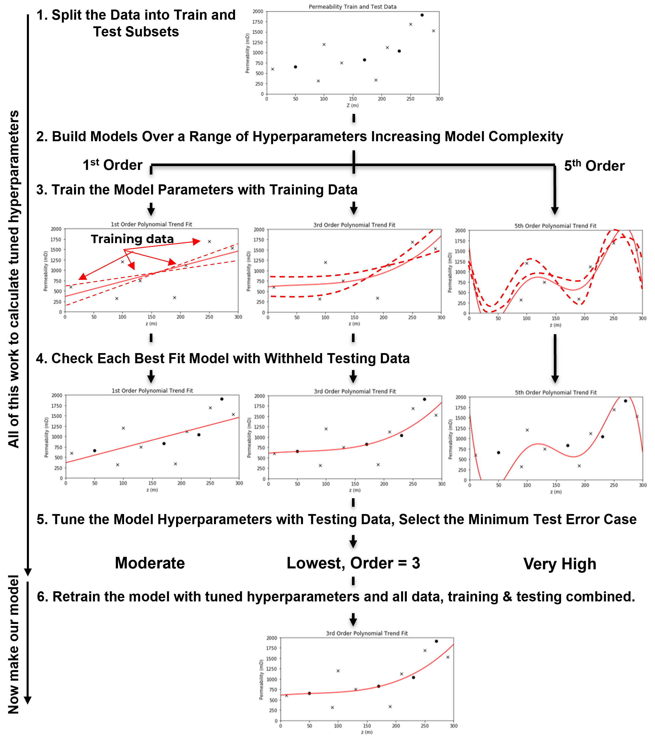
Standard predictive machine learning modeling workflow.

Let’s walk through the key steps,

Train and Test Split - divide the available data into mutually exclusive, exhaustive subsets: a training set and a testing set.

typically, 15%–30% of the data is held out for testing
the remaining 70%–85% is used for training the model

Define a range of hyperparameter(s) values to explore, ranging from,

simple models with low flexibility
to complex models with high flexibility

\(\quad\) This step may involve tuning multiple hyperparameters, in which case efficient sampling methods (e.g., grid search, random search, or Bayesian optimization) are often used.

Train Model Parameters for Each Hyperparameter Setting - for each set of hyperparameters, train a model on the training data. This yields:

a suite of trained models, each with different complexity
each model has parameters optimized to minimize error on the training data

Evaluate Each Model on the Withheld Testing Data - using the testing data,

evaluate how each trained model performs on unseen data
summarize prediction error (for example, root mean square error (RMSE), mean absolute error (MAE), classification accuracy) for each model

Select the Hyperparameters That Minimize Test Error - this is the hyperparameter tuning step:

choose the model hyperparaemter(s) that performs best on the test data
these are your tuned hyperparameters

Retrain the Final Model on All Data Using Tuned Hyperparameters - now that the best model complexity has been identified,

retrain the model using both the training and test sets
this maximizes the amount of data used for final model parameter estimation
the resulting model is the one you deploy in real-world applications

Common Questions About the Model Training and Tuning Workflow#

As a professor, I often hear these questions when I introduce the above machine learning model training and tuning workflow.

What is the main outcome of steps 1–5? - the only reliable outcome is the tuned hyperparameters.

\(\quad\) we do not use the model trained in step 3 or 4 directly, because it was trained without access to all available data. Instead, we retrain the final model using all data with the selected hyperparameters.

Why not train the model on all the data from the beginning? - because if we do that, we have no independent way to evaluate the model’s generalization. A very complex model can easily overfit—fitting the training data perfectly, but performing poorly on new, unseen data.

\(\quad\) overfitting happens when model flexibility is too high—it captures noise instead of the underlying pattern. Without a withheld test set, we can’t detect this.

This workflow for training and tuning predictive machine learning models is,

an empirical, cross-validation-based process
a practical simulation of real-world model use
a method to identify the model complexity that best balances fit and generalization

I’ve said model parameters and model hyperparameters a bunch of times, so I owe you their definitions.

Model Parameters and Model Hyperparameters#

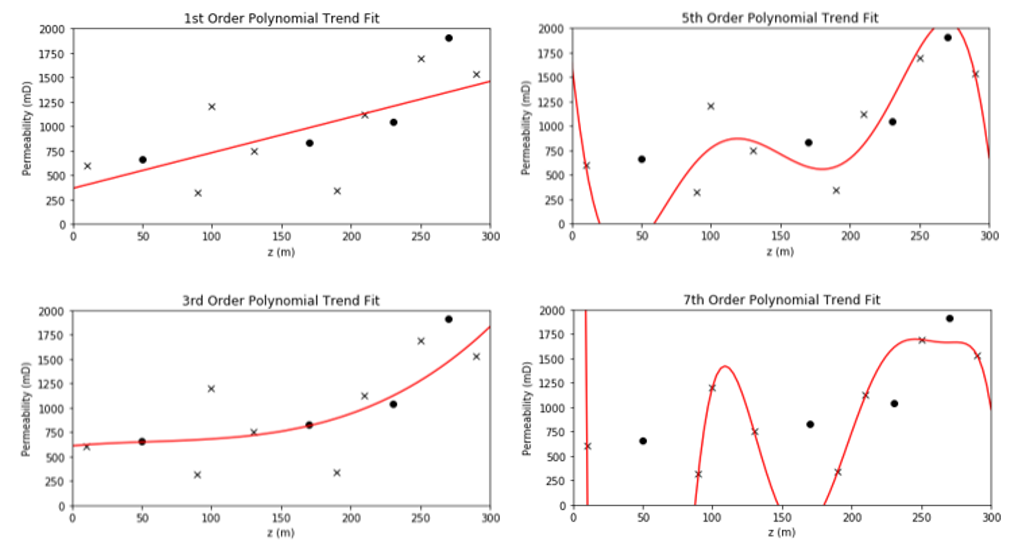
Model parameters are fit during training phase to minimize error at the training data, i.e., model parameters are trained with training data and control model fit to the data. For example,

for the polynomial predictive machine learning model from the machine learning workflow example above, the model parameters are the polynomial coefficients, e.g., \(b_3\), \(b_2\), \(b_1\) and \(c\) (often called \(b_0\)) for the third order polynomial model.

Model parameters are adjusted to fit of the model to the data, i.e., model parameters are trained to minimize error over the training data (x markers).

Model hyperparameters are very different. They do not constrain the model fit to the data directly, instead they constrain the model complexity. The model hyperparameters are selected (call tuning) to minimize error at the withheld testing data. Going back to our polynomial predictive machine learning example, the choice of polynomial order is the model hyperparameter.

Model hyperparameters are adjusted to change the model complexity / flexibility, i.e., model hyperparameters are tuned to minimize error over the withheld testing data (solid circles).

Model parameters vs. model hyperparameters

Model parameters control the model fit and are trained with training data. Model hyperparameters control the model complexity and are tuned with testing data.

Regression and Classification#

Before we proceed, we need to define regression and classification.

Regression - a predictive machine learning model where the response feature(s) is continuous.
Classification - a predictive machine learning model where the response feature(s) is categorical.

It turns out that for each of these we need to build different models and use different methods to score these models.

for the remainder of this discussion we will focus on regression, but in later chapters we introduce classification models as well.

Now, to better understand predictive machine learning model tuning, i.e., the empirical approach to tune model complexity to minimize testing error, we need to understand the sources of testing error.

the causes of the thing that we are attempting to minimize!

Sources of Predictive Machine Learning Testing Error#

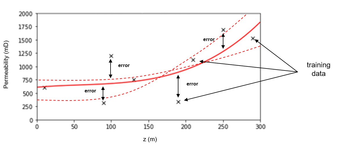
Mean square error (MSE) is a standard way to express error. Mean squared error is known as a norm because we at taking a vector of error (over all of the data) and summarizing with a single, non-negative value.

specifically MSER is the L2 norm because the errors are squared before they are summed,
the L2 norm has a lot of nice properties including a continuous error function that can be differentiated over all values of error, but it is sensitive to data outliers that may have a disproportionate impact on the sum of the squares. More about this later.

\[ MSE = \frac{1}{n} \sum_{i=1}^{n} \left( y_i - \hat{y}_i \right)^2 \]

where \(y_i\) is the actual observation of the response feature and \(\hat{y}_i\) is the model estimate over data indexed, \(i = 1,\ldots,n\). The \(\hat{y}_i\) is estimated with our predictive machine learning model with a general form,

\[ \hat{y}_i = \hat{f}(x^1_i, \ldots , x^m_i) \]

where \(\hat{f}\) is our predictive machine learning model and \(x^1_i, \ldots , x^m_i\) are the predictor feature values for the \(i^{th}\) data.

Of course, MSE can be calculated over training data and this is often the loss function that we minimize for training the model parameters for regression models.

\[ MSE_{train} = \frac{1}{n_{train}} \sum_{i=1}^{n_{train}} \left( y_i - \hat{y}_i \right)^2 \]

and MSE can be calculated over the withheld testing data for hyperparameter tuning of regression models.

If we take the \(MSE_{test}\),

\[ MSE_{test} = \frac{1}{n_{test}} \sum_{i=1}^{n_{test}} \left( y_i - \hat{f}(x^1_i, \ldots , x^m_i) \right)^2 \]

but we pose it as the expected test square error we get this expectation form,

\[ E \left[ \left( y_0 - \hat{f}(x^1_0, \ldots , x^m_0) \right)^2 \right] \]

where we use the \(_0\) notation to indicate data samples not in the training dataset split, but in the withheld testing split. We can expand the quadratic and group the terms to get this convenient decomposition of expect test square error into three additive sources (derivation is available in Hastie et al., 2009,

Model error in testing with three additive components, model variance, model bias and irreducible error.

Let’s explain these three additive sources of error over test data, i.e., our best representation of the error we expect in the real-world use of our model to predict for cases not used to train the model,

Model Variance - is error due to sensitivity to the dataset, for example a simple model like linear regression does not change much if we change the training data, but a more complicated model like a fifth order polynomial model will jump around a lot as we change the training data.

\(\quad\) More model complexity tends to increase model variance.

Model Bias - is error due to using an approximate model, i.e., the model is too simple to fit the natural phenomenon. A very simple model is inflexible and will generally have higher model bias while a more complicated model is flexible enough to fit the data and will have lower model bias.

\(\quad\) More model complexity tends to descrease model bias.

Irreducible Error - is due to missing and incomplete data. There may be important features that were not sampled, or ranges of feature values that were not sampled. This is the error due to data limitations that cannot be address by the machine learning model hyperparameter tuning for optimum complexity; therefore, irreducible error is constant over the range of model complexity.

\(\quad\) More model complexity should not change irreducible error.

Now we can take these three additive sources of error and produce an instructive, schematic plot,

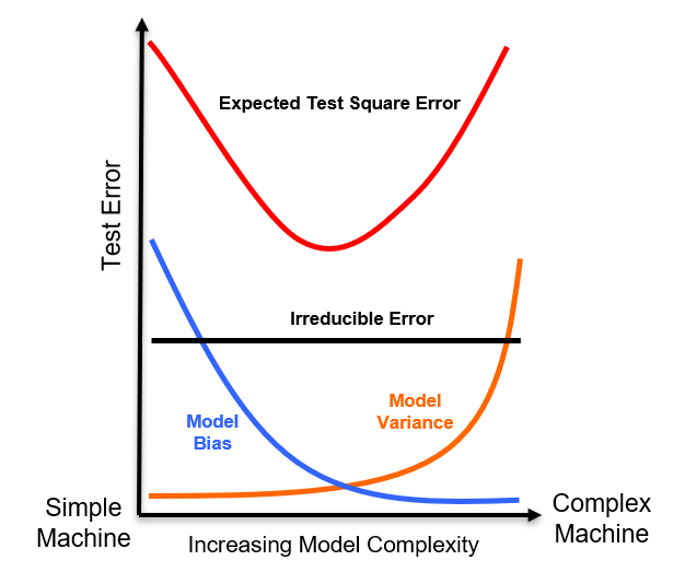
Model error in testing vs. model complexity with three additive error components, model variance, model bias and irreducible error.

From this plot we can observe, the model bias-variance trade off,

testing error is high for low complexity models due to high model bias
testing error is high for high complexity models due to high model variance

So hyperparameter tuning is an optimization of the model bias-variance trade off. Wwe select the model complexity via hyperparameters that results in a model that is not,

underfit - too simple, too inflexible to fit the natural phenomenon
overfit - too complicated, too flexible and is too sensitive to the data

Now, let’s get into more details about under and overfit machine learning models.

Underfit and Overfit Models#

First visualize underfit and overfit first with a simple prediction problem with one predictor feature and one response feature, here’s a model that is too simple (left) and a model that is too complicated (right).

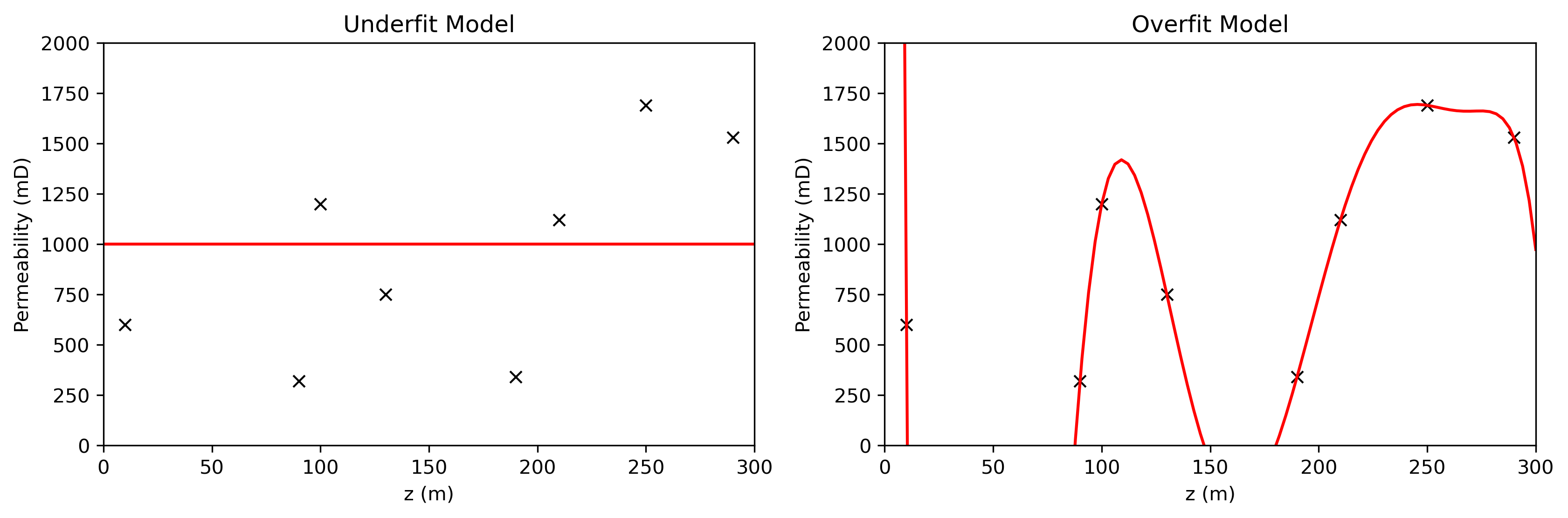
Example underfit model (left), a model that is too simple / inflexible and overfit model (right), a model that is too complicated / flexible.

Some observations,

the simple model is not sufficiently flexible to fit the data, this is likely an underfit model
the overfit model perfectly fits all of the training data but is too noisy away from the training data and is likely an overfit model

To better understand the difference, we can now plot the training error alongside the previously shown testing error curve, illustrating how both change with model complexity.

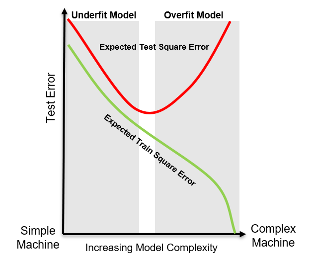
Model error in training and testing vs. model complexity with illustration of under- and overfit model regions.

From the plot, we can make the following observations:

Training Error – as model complexity increases, training error consistently decreases. With sufficient flexibility, the model can eventually fit the training data perfectly, driving training error to zero.
Testing Error – testing error is composed of bias, variance, and irreducible error. The interplay between bias and variance leads to a trade-off, resulting in an optimal model complexity that minimizes testing error.

Based on these observations, we can characterize underfitting and overfitting as follows:

Underfitting - occurs when a model is too simple to capture the underlying patterns in the data. Such models fail to generalize well and tend to show high training and testing errors. As complexity increases, testing error decreases.
Overfitting - occurs when a model is too complex and captures not only the underlying data patterns but also the noise. While training error continues to decrease, testing error starts to increase due to poor generalization. These models can give a false impression of strong performance, misleading us into thinking we understand the system better than we do.

More About Training and Testing Splits#

A critical part of the machine learning training and tuning workflow is the training and testing data split. Here is some more considerations about training and testing data splits,

Proportion Withheld for Testing#

Meta studies have identified that between 15% and 30% withheld for testing is typically optimum. To understand the underlying trade-off imagine these end members,

withhold 2% of the data for testing, then we will have a lot of training data to train the model very well, but too few testing data to test our model over a range of prediction cases.
withhold 98% of the data for test, then with only 2% of the data available for training we will do a very good job testing our very poor model.

The proportion to withhold for testing is a trade off between building a good model and testing this model well with a wide range of prediction cases.

Other Cross Validation Methods#

The train and test workflow above known as a cross validation or hold out approach, but there are many other methods for model training and testing,

k-fold Cross Validation (K-fold CV) - we divide the data into k mutually exclusive, exhaustive equal size sets (called folds) for repeat the model train and test k times with each fold having a turn being withheld testing data while the remainder is training data.
Leave-One-Out Cross Validation (LOO CV) - we loop over all data, each time we assign the one datum as the testing data and train on the remainder n-1 data.
Leave-p-Out Cross Validation (LpO-CV) - we assign a integer p < n and then loop over the combinatorial of possible cases with p withheld testing data. Since we consider all possible cases, this is an exhaustive cross validation approach.

For each of the above folds or in general, training and testing dataset combinations, we calculate the error norm

then we average the error norm over the folds to provide a single error for hyperparameter tuning
this method removes the sensitivity to the exact train and test split so it is often seen as more robust than regular hold out methods.

The choice of proportion of the data to withhold for testing varies by the the cross validation method,

for k-fold cross validation the proportion of testing is implicit to the choice of k, for k = 3, 33% of data are withheld for each fold and for k=5, 20% of data are withheld for each fold
for leave-one-out cross validation the proportion of testing is \(\frac{1}{n}\)
for leave-p-out cross validation the proportion of testing is \(\frac{p}{n}\)

Train, Validate and Test Split#

There is an alternative approach with three exhaustive, mutually exclusive subsets of the data

training data - subset is the same as train above and is used to train the model parameters
validate data - subset is like testing subset for the train and test split method above and is used to tune the model hyperparameters
testing data - subset is applied to check the final model trained on all the data with the tuned hyperparameters

The train, validate and test split philosophy is that this final model check is performed with data that was not involved with model construction, including training model parameters nor tuning model hyperparameters. There are two reasons that I push back on this method,

circular quest of perfect model validation - what do we do if we don’t quite like the performance in this testing phase, do we have a fourth subset for another test? and a fifth subset? and a sixth subset? ad infinitum?
we must train the deployed model with all data - we can never deploy a model that is not trained with all available data; therefore, we will still have to train with the test subset to get our final model?
reducing modeling training and tuning performance - the third data split for the testing phase reduces the data available for model training and tuning reducing the perforamnce of these critical steps.

Spatial Fair Train and Test Splits#

Dr. Julian Salazar suggested that for spatial prediction problems that random train and test split may not fair. He proposed a fair train and test split method for spatial prediction models that splits the data based on the difficulty of the planned use of the model. Prediction difficulty is related to kriging variance that accounts for spatial continuity and distance offset. For example,

if the model will be used to impute data with small offsets from available data then construct a train and test split with train data close to test data
if the model will be used to predict a large distance offsets then perform splits the result is large offsets between train and test data.

With this method the tuned model may vary based on the planned real-world use for the model.

Ethical and Professional Practice Concerns with Data Science#

To demonstrate concerns with data science consider this example, Rideiro et al. (2016) trained a logistic regression classifier with 20 wolf and dog images to detect the difference between wolves and dogs.

the input is a photo of a dog or wolf and the output is the probability of dog and the compliment, the probability of wolf
the model worked well until this example here (see the left side below),

Example dog misclassified as a wolf (left) and pixels that resulted in this misclassification (right), image taken from Rideiro et al. (2016).

where this results in a high probability of wolf. Fortunately the authors were able to interrogate the model and determine the pixels that had the greatest influence of the model’s determination of wolf (see the right side above). What happened?

they trained a model to check for snow in the background. As a Canadian, I can assure you that many photos of wolves are in our snow filled northern regions of our country, while many dogs are photographed in grassy yards.

The problems with machine learning are,

interpretability may be low with complicated models
application of machine learning may become routine and trusted

This is a dangerous combination, as the machine may become a trusted unquestioned authority. Rideiro and others state that they developed the problem to demonstrate this, but does it actually happen? Yes. I advised a team of students that attempted to automatically segment urban vs. rural environments from time lapse satellite photographs to build models of urban development. The model looked great, but I asked for an additional check with a plot of the by-pixel classification vs. pixel color. The results was a 100% correspondence, i.e., the model with all of it’s complicated convolution, activation, pooling was only looking for grey and tan pixels often associated with roads and buildings.

I’m not going to say, ‘Skynet’, oops I just did, but just consider these thoughts:

New power and distribution of wealth by concentrating rapid inference with big data as more data is being shared
Trade-offs that matter to society while maximizing a machine learning objective function may be ignored, resulting in low interpretability
Societal changes, disruptive technologies, post-labor society
Non-scientific results such as Clever Hans effect with models that learn from tells in the data rather than really learning to perform the task resulting catastrophic failures

I don’t want to be too negative and to take this too far. Full disclosure, I’m the old-fashioned professor that thinks we should put of phones in our pockets, walk around with our heads up so we can greet each other and observe our amazing environments and societies. One thing that is certain, data science is changing society in so many ways and as Neil Postman in Technopoly)

Neil Postman’s Quote for Technopoly

“Once a technology is admitted, it plays out its hand.”

Comments#

This was a basic description of machine learning concepts. Much more could be done and discussed, I have many more resources. Check out my shared resource inventory and the YouTube lecture links at the start of this chapter with resource links in the videos’ descriptions.

I hope this was helpful,

Michael

About the Author#

Michael Pyrcz is a professor in the Cockrell School of Engineering, and the Jackson School of Geosciences, at The University of Texas at Austin, where he researches and teaches subsurface, spatial data analytics, geostatistics, and machine learning. Michael is also,

the principal investigator of the Energy Analytics freshmen research initiative and a core faculty in the Machine Learn Laboratory in the College of Natural Sciences, The University of Texas at Austin
an associate editor for Computers and Geosciences, and a board member for Mathematical Geosciences, the International Association for Mathematical Geosciences.

Michael has written over 70 peer-reviewed publications, a Python package for spatial data analytics, co-authored a textbook on spatial data analytics, Geostatistical Reservoir Modeling and author of two recently released e-books, Applied Geostatistics in Python: a Hands-on Guide with GeostatsPy and Applied Machine Learning in Python: a Hands-on Guide with Code.

All of Michael’s university lectures are available on his YouTube Channel with links to 100s of Python interactive dashboards and well-documented workflows in over 40 repositories on his GitHub account, to support any interested students and working professionals with evergreen content. To find out more about Michael’s work and shared educational resources visit his Website.

Want to Work Together?#

I hope this content is helpful to those that want to learn more about subsurface modeling, data analytics and machine learning. Students and working professionals are welcome to participate.

Want to invite me to visit your company for training, mentoring, project review, workflow design and / or consulting? I’d be happy to drop by and work with you!
Interested in partnering, supporting my graduate student research or my Subsurface Data Analytics and Machine Learning consortium (co-PIs including Profs. Foster, Torres-Verdin and van Oort)? My research combines data analytics, stochastic modeling and machine learning theory with practice to develop novel methods and workflows to add value. We are solving challenging subsurface problems!
I can be reached at mpyrcz@austin.utexas.edu.

I’m always happy to discuss,