

Machine Learning Python Code Snippets#
Michael J. Pyrcz, Professor, The University of Texas at Austin
Twitter | GitHub | Website | GoogleScholar | Geostatistics Book | YouTube | Applied Geostats in Python e-book | Applied Machine Learning in Python e-book | LinkedIn
Chapter of e-book “Applied Machine Learning in Python: a Hands-on Guide with Code”.
Cite this e-Book as:
Pyrcz, M.J., 2024, Applied Machine Learning in Python: A Hands-on Guide with Code [e-book]. Zenodo. doi:10.5281/zenodo.15169139 ![]()
The workflows in this book and more are available here:
Cite the MachineLearningDemos GitHub Repository as:
Pyrcz, M.J., 2024, MachineLearningDemos: Python Machine Learning Demonstration Workflows Repository (0.0.3) [Software]. Zenodo. DOI: 10.5281/zenodo.13835312. GitHub repository: GeostatsGuy/MachineLearningDemos ![]()
By Michael J. Pyrcz
© Copyright 2024.
This chapter is a set of Machine Learning Python Code Snippets to help folks build machine learning workflows in Python.
YouTube Lecture: check out my live code walk-throughs in my data science basics in Python playlist:
These walkthrough support of my courses,
on YouTube with linked well-documented Python workflows and interactive dashboards. My goal is to share accessible, actionable, and repeatable educational content. If you want to know about my motivation, check out Michael’s Story.
Motivation#
I taught a high school hackathon with great students from all over Texas and beyond and I felt that they could use some additional resources in the form of a code snippets to help them over the hurdles of completing their first data science workflow in Python.
Remember the definition of a code snippet is,
a small, reusable section of code that programmers can quickly insert into a larger codebase
My goal is to,
provide a set of minimum, simple code snippets to accomplish basic data science modeling build steps
avoid fancy additions, like automatic diagnostics and plotting that are specific to the problem setting that will break with new data
Therefore, improvements and additions to provide diagnostic outputs and plots are highly recommended.
Structure#
This is not a workflow!
These are alphabetically ordered code snippets and not a complete workflow. Please do not attempt to run this chapter in sequence.
In order to run the snippets we need to first,
Import some python packages
Declare a couple of convenience functions
Load some data to demonstrate the code snippets
After we load the data the remaining codes with be in alphabetical and not any logical workflow order for ease of search and retrieval.
Import Required Packages#
We need some standard packages. These should have been installed with Anaconda 3.
import numpy as np                                            # arrays
import pandas as pd                                           # dataframes
import matplotlib.pyplot as plt                               # plotting
from matplotlib.ticker import (MultipleLocator, AutoMinorLocator, AutoLocator) # control of axes ticks
from statsmodels.stats.outliers_influence import variance_inflation_factor # variance inflation factor
from sklearn.impute import SimpleImputer                      # basic imputation method
from sklearn.experimental import enable_iterative_imputer     # required for MICE imputation
from sklearn.impute import IterativeImputer                   # MICE imputation
from sklearn.impute import KNNImputer                         # k-nearest neighbour imputation method
from sklearn.model_selection import train_test_split          # train and test split
from sklearn.linear_model import LinearRegression             # linear regression
from sklearn.preprocessing import StandardScaler              # standardize the features
from sklearn.preprocessing import MinMaxScaler                # min and max normalization
from sklearn.preprocessing import KBinsDiscretizer            # k-bin discretizer
from sklearn.neighbors import KNeighborsRegressor             # K-nearest neighbours
from sklearn.ensemble import RandomForestRegressor            # random forest method
from sklearn.feature_selection import mutual_info_regression  # mutual information
from sklearn.metrics import mean_absolute_error               # mean absolute error
from sklearn.metrics import normalized_mutual_info_score      # normalized mutual information
from sklearn import tree                                      # decision tree
from sklearn.tree import DecisionTreeRegressor                # regression tree
from sklearn.tree import plot_tree                            # plot the decision tree
from sklearn import metrics                                   # measures to check our models
import shap                                                   # Shapley values for feature ranking
plt.rc('axes', axisbelow=True)                                # set axes and grids in the background for all plots
import math
seed = 13
cmap = plt.cm.inferno                                         # a good colormap for folks with color perception issues
utcolor = '#BF5700'                                           # burnt orange, Hook'em!
IProgress not found. Please update jupyter and ipywidgets. See https://ipywidgets.readthedocs.io/en/stable/user_install.html
If you get a package import error, you may have to first install some of these packages. This can usually be accomplished by opening up a command window on Windows and then typing ‘python -m pip install [package-name]’. More assistance is available with the respective package docs.
Declare Functions#
Here’s the functions to improve code readability.
def add_grid():                                               # add grid lines
    plt.gca().grid(True, which='major',linewidth = 1.0); plt.gca().grid(True, which='minor',linewidth = 0.2) # add y grids
    plt.gca().tick_params(which='major',length=7); plt.gca().tick_params(which='minor', length=4)
    plt.gca().xaxis.set_minor_locator(AutoMinorLocator()); plt.gca().yaxis.set_minor_locator(AutoMinorLocator()) # turn on minor ticks
Load a Couple Datasets#
We load a couple of datasets,
df - an exhaustive data table as a pandas DataFrame
df_missing an data table with some missing data as a pandas DataFrame
ndarray_2D - a 2D array map as a NumPy ndarray
To demonstrat the methods below.
df = pd.read_csv(r"https://raw.githubusercontent.com/GeostatsGuy/GeoDataSets/master/unconv_MV_v4.csv") # load the data from my github repo
df_missing = pd.read_csv(r"https://raw.githubusercontent.com/GeostatsGuy/GeoDataSets/master/unconv_MV_missing.csv")
df_spatial = pd.read_csv(r"https://raw.githubusercontent.com/GeostatsGuy/GeoDataSets/master/12_sample_data.csv")
ndarray_2D = np.loadtxt("https://raw.githubusercontent.com/GeostatsGuy/GeoDataSets/master/12_AI.csv",
                     delimiter=",")
np.random.seed(seed=seed+7)                                     # set random number seed for reproducibility
df['Prod'] = df['Prod'] + np.random.normal(loc=0.0,scale=600.0,size=len(df)) # add noise to demonstrate overfit and hyperparameter tuning
Complete Some Basic Operations#
Here I complete some basic operations to ensure that the alphabetically sorted code snippets below have the inputs to avoid errors.
X = df.iloc[:,1:-1]; y = df.iloc[:,[-1]]                      # separate predictor and response, assumes response is the last features
X_missing = df_missing.iloc[:,1:-1]; y_missing = df_missing.iloc[:,[-1]] # separate predictor and response, assumes response is the last features
X_train, X_test, y_train, y_test = train_test_split(X, y,
                test_size=0.2, random_state=seed)             # train and test split
linear_model = LinearRegression().fit(X_train,y_train)        # instantiate and train linear regression model, no hyperparmeters
y_hat_train = linear_model.predict(X_train)                   # predict over the training data
y_hat_test = linear_model.predict(X_test)                     # predict over the training data
linear_1pred_model = LinearRegression().fit(X_train[['Por']].values,y_train) # linear regression model with only 1 predictor feature
linear_2pred_model = LinearRegression().fit(X_train[['Por','Brittle']].values,y_train) # linear regression model with only 1 predictor feature
OK, now we are ready to walk thorugh our alphabetically ordered code snippets.
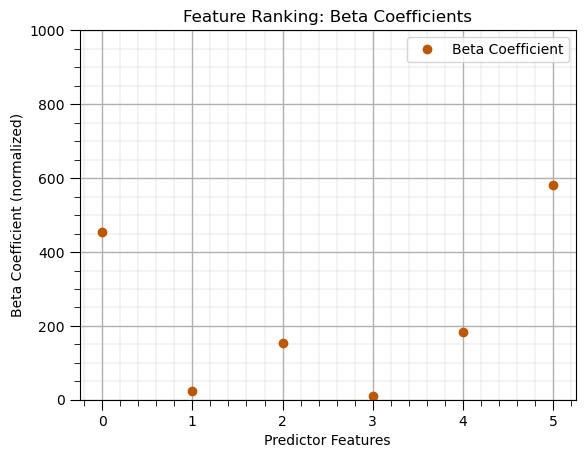
Beta, \(\beta\), Coefficients#
Feature importance based on the multilinear regression coefficients of the normalized features.
normalizer = MinMaxScaler()                                   # instantiate the min/max normalizer
norm_array = normalizer.fit_transform(X)                      # normalize the predictor features
X_norm = pd.DataFrame(norm_array, columns=X.columns)          # convert output to a DataFrame
beta_linear_model = LinearRegression().fit(X_norm,y)   # instantiate and train linear regression model, no hyperparmeters
beta_coef_df = pd.DataFrame({'Feature': list(X.columns),'Beta Coefficient': list(np.abs(linear_model.coef_.ravel()))})
beta_coef_df.plot(color=utcolor,style='o'); plt.xlabel('Predictor Features'); plt.ylabel('Beta Coefficient (normalized)'); plt.ylim(0,1000)
plt.title('Feature Ranking: Beta Coefficients'); add_grid(); plt.show()
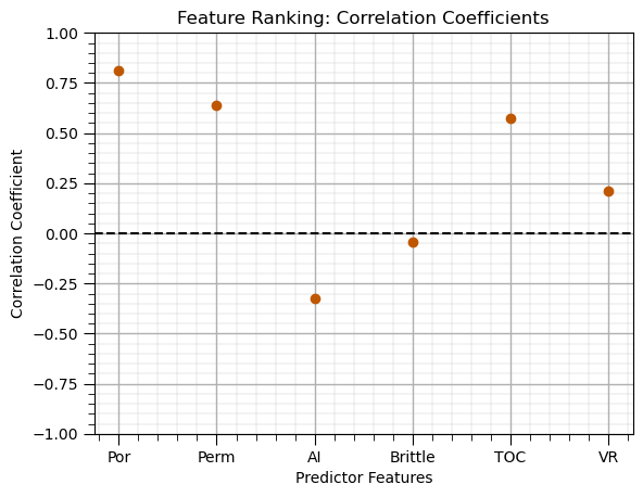
Correlation (Pearson product momment)#
correlations = df.corr().loc[X.columns, y.columns[0]]         # calculate correlation matrix and extract the pred. rows for the response column
correlations.plot(color=utcolor,style='o'); plt.xlabel('Predictor Features'); plt.ylabel('Correlation Coefficient'); plt.ylim(-1,1);
plt.title('Feature Ranking: Correlation Coefficients'); plt.axhline(y=0.0, color='black', linestyle='--'); add_grid(); plt.show()
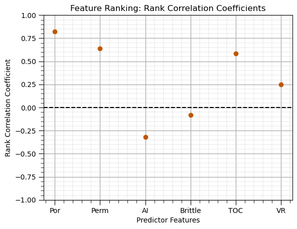
Correlation (Spearman rank)#
rank_correlations = df.corr(method='spearman').loc[X.columns, y.columns[0]] # calculate Spearman correlation with same method as Pearson above
rank_correlations.plot(color=utcolor,style='o'); plt.xlabel('Predictor Features'); plt.ylabel('Rank Correlation Coefficient'); plt.ylim(-1,1);
plt.title('Feature Ranking: Rank Correlation Coefficients'); plt.axhline(y=0.0, color='black', linestyle='--'); add_grid(); plt.show()
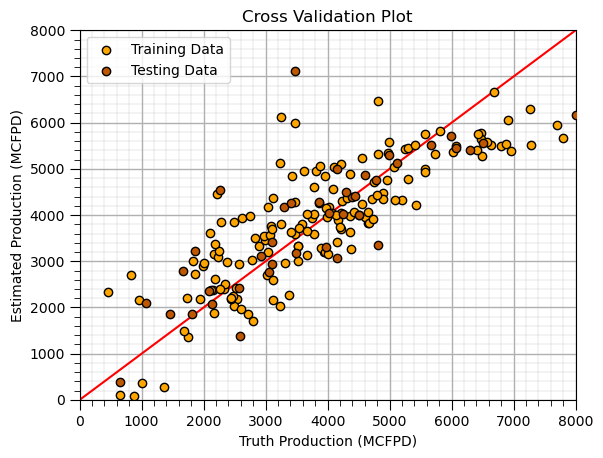
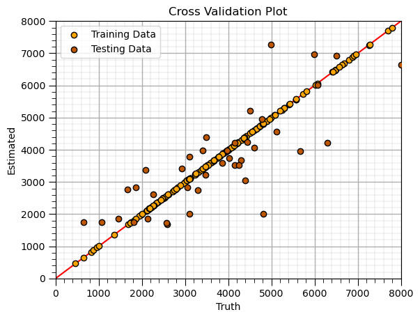
Cross Validation Plot (training and testing)#
plt.scatter(y_train,y_hat_train,color='orange',edgecolor='black',label=r'Training Data',zorder=10) # scatter plot
plt.scatter(y_test,y_hat_test,color=utcolor,edgecolor='black',label=r'Testing Data',zorder=10)
plt.ylabel('Estimated Production (MCFPD)'); plt.xlabel('Truth Production (MCFPD)'); plt.title('Cross Validation Plot'); plt.legend(loc = 'upper left')
plt.plot([0,8000],[0,8000],color='red'); plt.xlim(0,8000,); plt.ylim(0,8000); add_grid();
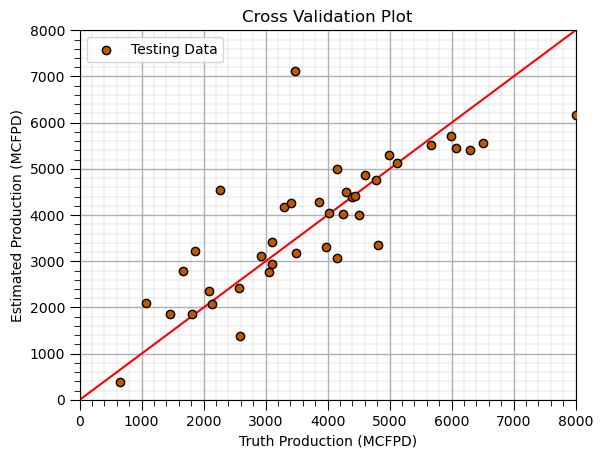
Cross Validation Plot (testing)#
plt.scatter(y_test,y_hat_test,color=utcolor,edgecolor='black',label=r'Testing Data',zorder=10) # scatter plot
plt.ylabel('Estimated Production (MCFPD)'); plt.xlabel('Truth Production (MCFPD)'); plt.title('Cross Validation Plot'); plt.legend(loc = 'upper left')
plt.plot([0,8000],[0,8000],color='red'); plt.xlim(0,8000,); plt.ylim(0,8000); add_grid()
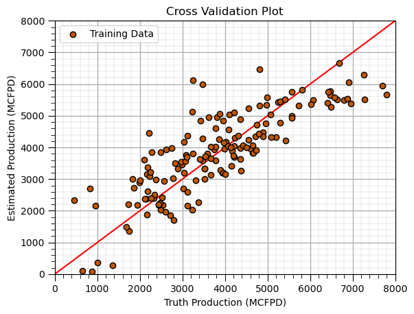
Cross Validation Plot (training)#
plt.scatter(y_train,y_hat_train,color=utcolor,edgecolor='black',label=r'Training Data',zorder=10) # scatter plot
plt.ylabel('Estimated Production (MCFPD)'); plt.xlabel('Truth Production (MCFPD)'); plt.title('Cross Validation Plot'); plt.legend(loc = 'upper left')
plt.plot([0,8000],[0,8000],color='red'); plt.xlim(0,8000,); plt.ylim(0,8000); add_grid();
DataFrame (add noise to a feature)#
I do this to experiment and make educational content, e.g., add noise to the response feature to demonstrate overfit.
df_temp = df.copy(deep=True)                                  # make a deep copy of the DataFrame
np.random.seed(seed=seed)                                     # set random seed for repeatability
df_temp['Prod'] = df_temp['Prod'] + np.random.normal(loc=0.0,scale=100.0,size=len(df_temp)) # add a feature of ones called 'Ones'
df_temp.head()
| Well | Por | Perm | AI | Brittle | TOC | VR | Prod | |
|---|---|---|---|---|---|---|---|---|
| 0 | 1 | 12.08 | 2.92 | 2.80 | 81.40 | 1.16 | 2.31 | 2154.457620 |
| 1 | 2 | 12.38 | 3.53 | 3.22 | 46.17 | 0.89 | 1.88 | 3199.991714 |
| 2 | 3 | 14.02 | 2.59 | 4.01 | 72.80 | 0.89 | 2.72 | 2742.009861 |
| 3 | 4 | 17.67 | 6.75 | 2.63 | 39.81 | 1.08 | 1.88 | 3927.738944 |
| 4 | 5 | 17.52 | 4.57 | 3.18 | 10.94 | 1.51 | 1.90 | 2343.080242 |
DataFrame (add a new feature/column)#
df_temp = df.copy(deep=True)                                  # make a deep copy of the DataFrame
df_temp['Ones'] = np.ones((len(df_temp)))                     # add a feature of ones called 'Ones'
df_temp.head()
| Well | Por | Perm | AI | Brittle | TOC | VR | Prod | Ones | |
|---|---|---|---|---|---|---|---|---|---|
| 0 | 1 | 12.08 | 2.92 | 2.80 | 81.40 | 1.16 | 2.31 | 2225.696687 | 1.0 |
| 1 | 2 | 12.38 | 3.53 | 3.22 | 46.17 | 0.89 | 1.88 | 3124.615076 | 1.0 |
| 2 | 3 | 14.02 | 2.59 | 4.01 | 72.80 | 0.89 | 2.72 | 2746.460169 | 1.0 |
| 3 | 4 | 17.67 | 6.75 | 2.63 | 39.81 | 1.08 | 1.88 | 3882.557711 | 1.0 |
| 4 | 5 | 17.52 | 4.57 | 3.18 | 10.94 | 1.51 | 1.90 | 2208.570072 | 1.0 |
DataFrame (make new)#
df_new = pd.DataFrame({'Ones':np.ones((100)),'Zeros':np.zeros((100))}) # make new DataFrame
df_new.head()
| Ones | Zeros | |
|---|---|---|
| 0 | 1.0 | 0.0 |
| 1 | 1.0 | 0.0 |
| 2 | 1.0 | 0.0 |
| 3 | 1.0 | 0.0 |
| 4 | 1.0 | 0.0 |
DataFrame (preview)#
Display the first ‘n’ rows of the DataFrame
df.head(n=13) # display the first n rows of the DataFrame
| Well | Por | Perm | AI | Brittle | TOC | VR | Prod | |
|---|---|---|---|---|---|---|---|---|
| 0 | 1 | 12.08 | 2.92 | 2.80 | 81.40 | 1.16 | 2.31 | 2225.696687 |
| 1 | 2 | 12.38 | 3.53 | 3.22 | 46.17 | 0.89 | 1.88 | 3124.615076 |
| 2 | 3 | 14.02 | 2.59 | 4.01 | 72.80 | 0.89 | 2.72 | 2746.460169 |
| 3 | 4 | 17.67 | 6.75 | 2.63 | 39.81 | 1.08 | 1.88 | 3882.557711 |
| 4 | 5 | 17.52 | 4.57 | 3.18 | 10.94 | 1.51 | 1.90 | 2208.570072 |
| 5 | 6 | 14.53 | 4.81 | 2.69 | 53.60 | 0.94 | 1.67 | 4353.192212 |
| 6 | 7 | 13.49 | 3.60 | 2.93 | 63.71 | 0.80 | 1.85 | 3516.494383 |
| 7 | 8 | 11.58 | 3.03 | 3.25 | 53.00 | 0.69 | 1.93 | 2083.845221 |
| 8 | 9 | 12.52 | 2.72 | 2.43 | 65.77 | 0.95 | 1.98 | 2775.906282 |
| 9 | 10 | 13.25 | 3.94 | 3.71 | 66.20 | 1.14 | 2.65 | 2966.741947 |
| 10 | 11 | 15.04 | 4.39 | 2.22 | 61.11 | 1.08 | 1.77 | 4022.323780 |
| 11 | 12 | 16.19 | 6.30 | 2.29 | 49.10 | 1.53 | 1.86 | 4799.763575 |
| 12 | 13 | 16.82 | 5.42 | 2.80 | 66.65 | 1.17 | 1.98 | 3616.427242 |
DataFrame (rename a feature/column)#
df_temp = df.copy(deep=True)                                  # make a deep copy of the DataFrame
df_temp.rename(columns={'Por':'Porosity (%)'},inplace=True)   # rename 'Por' features as 'Porosity'
df_temp.head()
| Well | Porosity (%) | Perm | AI | Brittle | TOC | VR | Prod | |
|---|---|---|---|---|---|---|---|---|
| 0 | 1 | 12.08 | 2.92 | 2.80 | 81.40 | 1.16 | 2.31 | 2225.696687 |
| 1 | 2 | 12.38 | 3.53 | 3.22 | 46.17 | 0.89 | 1.88 | 3124.615076 |
| 2 | 3 | 14.02 | 2.59 | 4.01 | 72.80 | 0.89 | 2.72 | 2746.460169 |
| 3 | 4 | 17.67 | 6.75 | 2.63 | 39.81 | 1.08 | 1.88 | 3882.557711 |
| 4 | 5 | 17.52 | 4.57 | 3.18 | 10.94 | 1.51 | 1.90 | 2208.570072 |
DataFrame (remove features/columns)#
df_temp = df.copy(deep=True)                                  # make a deep copy of the DataFrame
df_temp.drop(columns=['Well','Por','AI'],inplace=True)        # remove features 'Well','Por' and 'AI'
df_temp.head()
| Perm | Brittle | TOC | VR | Prod | |
|---|---|---|---|---|---|
| 0 | 2.92 | 81.40 | 1.16 | 2.31 | 2225.696687 |
| 1 | 3.53 | 46.17 | 0.89 | 1.88 | 3124.615076 |
| 2 | 2.59 | 72.80 | 0.89 | 2.72 | 2746.460169 |
| 3 | 6.75 | 39.81 | 1.08 | 1.88 | 3882.557711 |
| 4 | 4.57 | 10.94 | 1.51 | 1.90 | 2208.570072 |
DataFrame (remove samples/rows)#
df_temp = df.copy(deep=True)                                  # make a deep copy of the DataFrame
df_temp = df_temp.drop(df.index[[0, 2, 4]])                   # removes samples 0, 2 and 4
df_temp.head()
| Well | Por | Perm | AI | Brittle | TOC | VR | Prod | |
|---|---|---|---|---|---|---|---|---|
| 1 | 2 | 12.38 | 3.53 | 3.22 | 46.17 | 0.89 | 1.88 | 3124.615076 |
| 3 | 4 | 17.67 | 6.75 | 2.63 | 39.81 | 1.08 | 1.88 | 3882.557711 |
| 5 | 6 | 14.53 | 4.81 | 2.69 | 53.60 | 0.94 | 1.67 | 4353.192212 |
| 6 | 7 | 13.49 | 3.60 | 2.93 | 63.71 | 0.80 | 1.85 | 3516.494383 |
| 7 | 8 | 11.58 | 3.03 | 3.25 | 53.00 | 0.69 | 1.93 | 2083.845221 |
DataFrame (remove samples/rows by condition)#
df_temp = df.copy(deep=True)                                  # make a deep copy of the DataFrame
df_temp = df_temp[df_temp['Por'] > 13.0]                      # remove all samples with 'Por' <= 13%
df_temp.head()
| Well | Por | Perm | AI | Brittle | TOC | VR | Prod | |
|---|---|---|---|---|---|---|---|---|
| 2 | 3 | 14.02 | 2.59 | 4.01 | 72.80 | 0.89 | 2.72 | 2746.460169 |
| 3 | 4 | 17.67 | 6.75 | 2.63 | 39.81 | 1.08 | 1.88 | 3882.557711 |
| 4 | 5 | 17.52 | 4.57 | 3.18 | 10.94 | 1.51 | 1.90 | 2208.570072 |
| 5 | 6 | 14.53 | 4.81 | 2.69 | 53.60 | 0.94 | 1.67 | 4353.192212 |
| 6 | 7 | 13.49 | 3.60 | 2.93 | 63.71 | 0.80 | 1.85 | 3516.494383 |
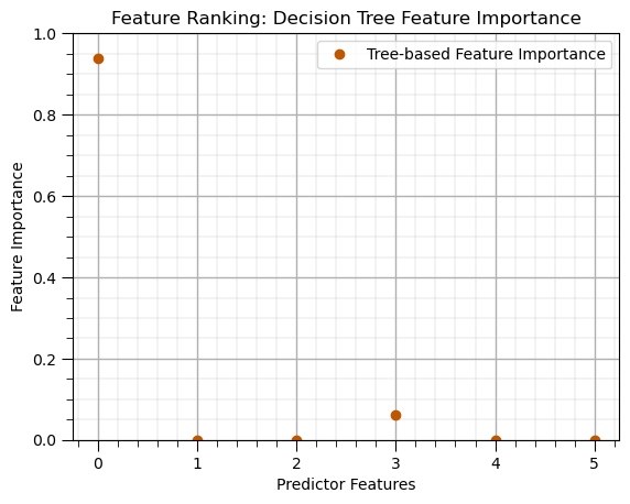
Decision Tree (feature importance)#
leaf_node = 5                                                 # decision tree model hyperparameters
tree_model = tree.DecisionTreeRegressor(max_leaf_nodes=leaf_node).fit(X_train,y_train) # instantiate the prediction model

beta_coef_df = pd.DataFrame({'Feature': list(X.columns),'Tree-based Feature Importance': list(tree_model.feature_importances_.ravel())})
beta_coef_df.plot(color=utcolor,style='o'); plt.xlabel('Predictor Features'); plt.ylabel('Feature Importance'); plt.ylim(0,1)
plt.title('Feature Ranking: Decision Tree Feature Importance'); add_grid(); plt.show()
Decision Tree (prediction at testing data)#
Apply our model to predict at withheld testing data.
leaf_node = 5                                                 # decision tree model hyperparameters
tree_model = tree.DecisionTreeRegressor(max_leaf_nodes=leaf_node).fit(X_train,y_train) # instantiate the prediction model
y_test_temp = y_test.copy(deep=True)
y_test_temp['Estimated Prod'] = tree_model.predict(X_test)    # predict over the training data
y_test_temp.head()
| Prod | Estimated Prod | |
|---|---|---|
| 179 | 656.507448 | 2218.196237 |
| 155 | 3110.245382 | 2218.196237 |
| 23 | 2581.359826 | 2218.196237 |
| 159 | 6498.151446 | 6482.917835 |
| 96 | 4148.822923 | 4297.451039 |
Decision Tree (prediction at training data)#
Apply our model to predict at the retained training data.
leaf_node = 5                                                 # decision tree model hyperparameters
tree_model = tree.DecisionTreeRegressor(max_leaf_nodes=leaf_node).fit(X_train,y_train) # instantiate the prediction model
y_train_temp = y_train.copy(deep=True)
y_train_temp['Estimated Prod'] = tree_model.predict(X_train)  # predict over the training data
y_train_temp.head()
| Prod | Estimated Prod | |
|---|---|---|
| 125 | 3750.106623 | 4297.451039 |
| 68 | 4644.717576 | 4297.451039 |
| 69 | 1991.991593 | 2218.196237 |
| 108 | 6688.360827 | 6482.917835 |
| 131 | 5076.638358 | 4297.451039 |
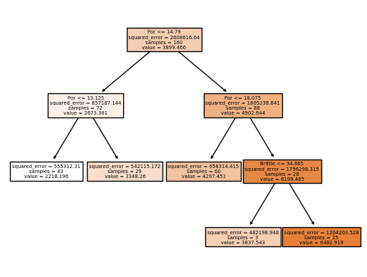
Decision Tree (train)#
Train model parameters on training data with specified model hyperparameters
let’s look at the trained model parameters, by visualizing the trained decision tree.
leaf_node = 5                                                 # decision tree model hyperparameters
tree_model = tree.DecisionTreeRegressor(max_leaf_nodes=leaf_node).fit(X_train,y_train) # instantiate the prediction model
plot_tree(tree_model, feature_names=X_train.columns, filled=True); plt.show() # plot the decision tree
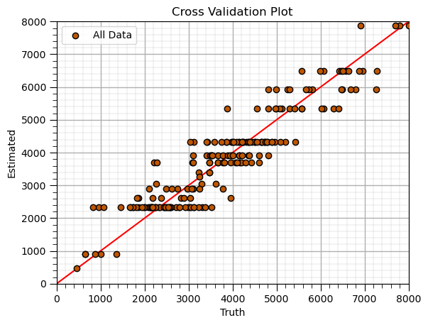
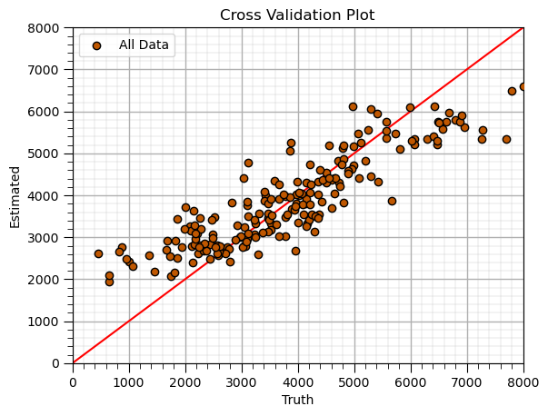
Decision Tree (retrain tuned model)#
Apply tuned hyperparameters and retrain the model with all the data.
this is the model that we will use for future predictions, real-world use
tuned_leaf_node = 15;                                         # decision tree model hyperparameters
tuned_tree_model = tree.DecisionTreeRegressor(max_leaf_nodes=tuned_leaf_node).fit(X,y) # instantiate the prediction model
y_hat = tuned_tree_model.predict(X)                           # predict over the testing cases
plt.scatter(y,y_hat,color=utcolor,edgecolor='black',label=r'All Data',zorder=10) # scatter plot
plt.ylabel('Estimated'); plt.xlabel('Truth'); plt.title('Cross Validation Plot'); plt.legend(loc = 'upper left')
plt.plot([0,8000],[0,8000],color='red'); plt.xlim(0,8000,); plt.ylim(0,8000)
add_grid();
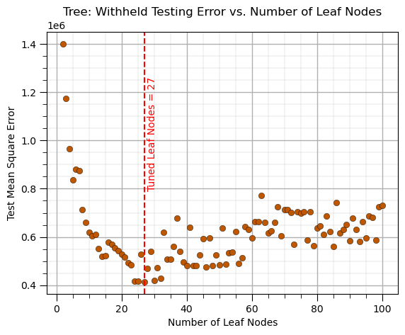
Decision Tree (tune/prune)#
Train model parameters on training data with a range of model hyperparameters, select the model hyperparameters with minimum error over the withheld testing data
This requires the following steps,
Loop over the hyperparameter(s) values,
train the model with the retained training data
predict at the withheld testing data
calculate the testing error
Select the hyperparameter that minimized the testing error
leaf_node = 2                                                 # set initial hyperparameter
MSE_tree_list = []; leaf_node_list = []                       # make lists to store the results
while leaf_node <= 100:                                       # loop over the number of leaf nodes hyperparameter
    tree_model = tree.DecisionTreeRegressor(max_leaf_nodes=leaf_node).fit(X_train,y_train) # instandiate and train the model
    y_hat_test = tree_model.predict(X_test)                   # predict over the testing cases
    MSE_tree = metrics.mean_squared_error(y_test,y_hat_test)  # calculate the MSE testing
    MSE_tree_list.append(MSE_tree)                            # add to the list of MSE
    leaf_node_list.append(leaf_node)                          # append leaf node to an array for plotting
    leaf_node = leaf_node + 1

tuned_leaf_nodes = leaf_node_list[np.argmin(MSE_tree_list)]           # get the k that minimizes the testing MSE

plt.subplot(111)
plt.scatter(leaf_node_list,MSE_tree_list,s=None, c=utcolor, alpha=1.0, linewidths=0.3, edgecolors="black") # plot testing MSE vs. hyperparameter
plt.axvline(x=tuned_leaf_nodes, color='red', linestyle='--')
plt.annotate('Tuned Leaf Nodes = ' + str(tuned_leaf_nodes),[tuned_leaf_nodes+1,0.8e6],color='red',rotation= 90)
plt.title('Tree: Withheld Testing Error vs. Number of Leaf Nodes'); plt.xlabel('Number of Leaf Nodes'); plt.ylabel('Test Mean Square Error')
add_grid()
Features Extraction (by name)#
Build a new DataFrame with only the selected predictor feature and the response feature
specify the selected predictor features
specify the response feature
build a list with both
make a new DataFrame with first the predictor features and then the response feature as the last column
selected_predictor_features = ['Por','Perm','AI','Brittle']   # set the selected predictor features
response_feature = ['Prod']                                   # set the response feature
features = selected_predictor_features + response_feature     # build a list of selected predictor and response features
df_selected = df.loc[:,features]                              # slice the DataFrame
df_selected.head()
| Por | Perm | AI | Brittle | Prod | |
|---|---|---|---|---|---|
| 0 | 12.08 | 2.92 | 2.80 | 81.40 | 2225.696687 |
| 1 | 12.38 | 3.53 | 3.22 | 46.17 | 3124.615076 |
| 2 | 14.02 | 2.59 | 4.01 | 72.80 | 2746.460169 |
| 3 | 17.67 | 6.75 | 2.63 | 39.81 | 3882.557711 |
| 4 | 17.52 | 4.57 | 3.18 | 10.94 | 2208.570072 |
Features Extraction (by number)#
Build a new DataFrame with only the selected predictor feature.
specify the selected predictor features
specify the response feature
build a list with both
make a new DataFrame with first the predictor features and then the response feature as the last column
selected_predictor_features = [1,2,3,4,7]                     # set the selected predictor features
df_selected_predictor = df.iloc[:,selected_predictor_features] # slice the DataFrame
df_selected_predictor.head()
| Por | Perm | AI | Brittle | Prod | |
|---|---|---|---|---|---|
| 0 | 12.08 | 2.92 | 2.80 | 81.40 | 2225.696687 |
| 1 | 12.38 | 3.53 | 3.22 | 46.17 | 3124.615076 |
| 2 | 14.02 | 2.59 | 4.01 | 72.80 | 2746.460169 |
| 3 | 17.67 | 6.75 | 2.63 | 39.81 | 3882.557711 |
| 4 | 17.52 | 4.57 | 3.18 | 10.94 | 2208.570072 |
Features Extraction (make X and y DataFrames)#
Build a two new DataFrames, one with only the selected predictor feature and the other with the response feature,
assuming that the last feature is the response feature
X = df.loc[:,['Por','AI','VR']]                               # extract the list the predictor feature by name
y = df.loc[:,['Prod']]                                        # extract the response feature
print('Predictor features: ' + str(X.columns.tolist()) + '\nResponse feature: ' + y.columns[0])
Predictor features: ['Por', 'AI', 'VR']
Response feature: Prod
Features Extraction (make X and y DataFrames assumed feature order)#
Build a two new DataFrames, one with only the selected predictor feature and the other with the response feature,
assuming that the last feature is the response feature
X = df.iloc[:,1:-1]; y = df.iloc[:,[-1]]                      # extract by assuming 2nd to 2nd last are predictors and last is response feature
print('Predictor features: ' + str(X.columns.tolist()) + '\nResponse feature: ' + y.columns[0])
Predictor features: ['Por', 'Perm', 'AI', 'Brittle', 'TOC', 'VR']
Response feature: Prod
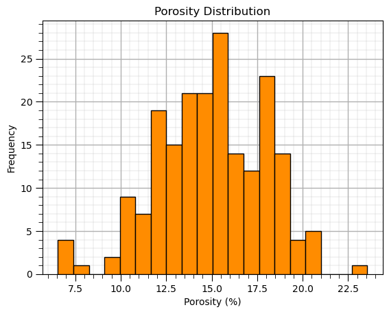
Histogram#
Simple histogram,
you can set the histogram limits by specifying the exact bins with a method like, np.linspace(min,max,n)
plt.hist(df['Por'],color='darkorange',edgecolor='black',bins=20); plt.xlabel('Porosity (%)'); plt.ylabel('Frequency') # histogram
plt.title('Porosity Distribution'); add_grid(); plt.show()
Histogram (normalized)#
A histogram with probability on the y axis and the sum of all bars is one, i.e., probability closure.
plt.hist(df['Por'],color='darkorange',edgecolor='black',weights = np.ones(len(df))/len(df),bins=20) # normalized histogram
plt.title('Porosity Distribution'); plt.xlabel('Porosity (%)'); plt.ylabel('Probability'); add_grid(); plt.show()
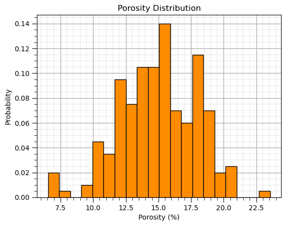
Image Plot#
im = plt.imshow(ndarray_2D,extent = [0,10000,0,10000],vmin=1500,vmax=6500,cmap = cmap) # plot of 2D ndarray, image or map feature
cbar = plt.colorbar(im, orientation="vertical", ticks=np.linspace(2500, 7500, 10)); plt.xlabel('X (m)'); plt.ylabel('Y (m)')
cbar.set_label(r'Acoustic Impedence ($\frac{kg}{m^3} \cdot \frac{m}{s} \cdot 10^3$)', rotation=270, labelpad=20)
plt.title('Acoustic Impedance'); plt.show()
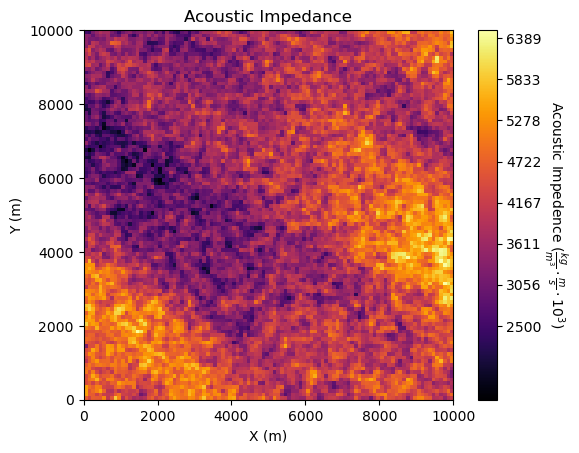
Image Plot (combined with location map)#
Superimpose multiple plots on top of each other,
use ‘zorder’ to place object in front of other objects, higher number is in front
make sure all objects are in the same plot space
im = plt.imshow(ndarray_2D,extent = [0,10000,0,10000],vmin=1500,vmax=6500,cmap = cmap,alpha=0.8,zorder=-1) # plot of 2D ndarray, image or map feature
sc = plt.scatter(df_spatial['X'],df_spatial['Y'],c=df_spatial['AI'],s=20,edgecolor='black',vmin=1500,vmax=6500,cmap = cmap,zorder=10)
cbar = plt.colorbar(im, orientation="vertical", ticks=np.linspace(2500, 7500, 10)); plt.xlabel('X (m)'); plt.ylabel('Y (m)')
cbar.set_label(r'Acoustic Impedence ($\frac{kg}{m^3} \cdot \frac{m}{s} \cdot 10^3$)', rotation=270, labelpad=20)
plt.title('Acoustic Impedance Image and Samples at Wells'); plt.show()

K-Nearest Neighbours (feature imputation)#
Feature imputation by estimating missing features with the nearest neighbours,
distance is accessed with all samples that have all features present in the sample with a missing feature
only one pass is applied, there is no iteration
not as robust as MICE is there is a lot of missing data, it does not learn the structure between the features to fill in missing data
knn_imputer = KNNImputer(n_neighbors=2, weights="uniform")    # instantiate Multiple Imputation by Chained Equations (MICE) imputer
X_imputed = knn_imputer.fit_transform(X_missing)              # train and apply MICE to impute the missing data
X_imputed = pd.DataFrame(X_imputed, columns=X_missing.columns,index=X_missing.index) # make imputed results into a DataFrame with same columns as X
X_imputed.describe()                                          # preview the DataFrame
| Por | LogPerm | AI | Brittle | TOC | VR | |
|---|---|---|---|---|---|---|
| count | 1000.000000 | 1000.000000 | 1000.000000 | 1000.000000 | 1000.000000 | 1000.000000 |
| mean | 14.924820 | 1.375450 | 2.982915 | 49.227565 | 1.014950 | 1.997420 |
| std | 2.999168 | 0.367557 | 0.557240 | 13.755077 | 0.480852 | 0.284183 |
| min | 5.400000 | 0.120000 | 0.960000 | -1.500000 | -0.250000 | 0.900000 |
| 25% | 12.846250 | 1.145000 | 2.590000 | 40.640000 | 0.700000 | 1.830000 |
| 50% | 15.035000 | 1.360000 | 3.010000 | 49.477500 | 1.007500 | 2.000000 |
| 75% | 17.012500 | 1.610000 | 3.330000 | 58.055000 | 1.370000 | 2.165000 |
| max | 24.650000 | 2.580000 | 4.700000 | 93.470000 | 2.710000 | 2.900000 |
K-Nearest Neighbours (prediction at testing data)#
Apply our model to predict at withheld testing data.
n_neighbours = 10; p = 2; weights = 'uniform'                 # KNN model hyperparameters
knn_model = KNeighborsRegressor(weights = weights, n_neighbors=n_neighbours, p = p).fit(X_train,y_train) # instantiate the prediction model
y_test_temp = y_test.copy(deep=True)
y_test_temp['Estimated Prod'] = knn_model.predict(X_test)     # predict over the training data
y_test_temp.head()
| Prod | Estimated Prod | |
|---|---|---|
| 179 | 656.507448 | 2303.626455 |
| 155 | 3110.245382 | 3774.108284 |
| 23 | 2581.359826 | 2321.644376 |
| 159 | 6498.151446 | 5713.166746 |
| 96 | 4148.822923 | 4108.942362 |
K-Nearest Neighbours (prediction at training data)#
Apply our model to predict at the retained training data.
n_neighbours = 10; p = 2; weights = 'uniform'                 # KNN model hyperparameters
knn_model = KNeighborsRegressor(weights = weights, n_neighbors=n_neighbours, p = p).fit(X_train,y_train) # instantiate the prediction model
y_train_temp = y_train.copy(deep=True)
y_train_temp['Estimated Prod'] = knn_model.predict(X_train)   # predict over the training data
y_train_temp.head()
| Prod | Estimated Prod | |
|---|---|---|
| 125 | 3750.106623 | 3974.087763 |
| 68 | 4644.717576 | 4226.039680 |
| 69 | 1991.991593 | 3165.041802 |
| 108 | 6688.360827 | 6336.236197 |
| 131 | 5076.638358 | 5332.676914 |
K-Nearest Neighbours (train)#
Train model parameters on training data with specified model hyperparameters
since K-nearest neighbours is a lazy learning model, there are no trained model parameters to display
instead we look at the cross validation plot
k = 1; p = 2; weights = 'uniform'                             # KNN model hyperparameters
neigh = KNeighborsRegressor(weights = weights, n_neighbors=k, p = p) # instantiate the prediction model
knn_model = neigh.fit(X_train,y_train)                        # train the model with the training data
y_train_hat = knn_model.predict(X_train)                      # predict over the testing cases
y_test_hat = knn_model.predict(X_test)                        # predict over the testing cases
plt.scatter(y_train,y_train_hat,color='orange',edgecolor='black',label=r'Training Data',zorder=10) # scatter plot
plt.scatter(y_test,y_test_hat,color=utcolor,edgecolor='black',label=r'Testing Data',zorder=10) # scatter plot
plt.ylabel('Estimated'); plt.xlabel('Truth'); plt.title('Cross Validation Plot'); plt.legend(loc = 'upper left')
plt.plot([0,8000],[0,8000],color='red'); plt.xlim(0,8000,); plt.ylim(0,8000)
add_grid()
K-Nearest Neighbours (retrain tuned model)#
Apply tuned hyperparameters and retrain the model with all the data.
this is the model that we will use for future predictions, real-world use
tuned_k = 15; p = 2; weights = 'uniform'                      # KNN model hyperparameters
knn_tuned_model = KNeighborsRegressor(weights = weights, n_neighbors=tuned_k, p = 2).fit(X,y) # retrain the tuned model with all data
y_hat = knn_tuned_model.predict(X)                            # predict over the testing cases
plt.scatter(y,y_hat,color=utcolor,edgecolor='black',label=r'All Data',zorder=10) # scatter plot
plt.ylabel('Estimated'); plt.xlabel('Truth'); plt.title('Cross Validation Plot'); plt.legend(loc = 'upper left')
plt.plot([0,8000],[0,8000],color='red'); plt.xlim(0,8000,); plt.ylim(0,8000); add_grid()
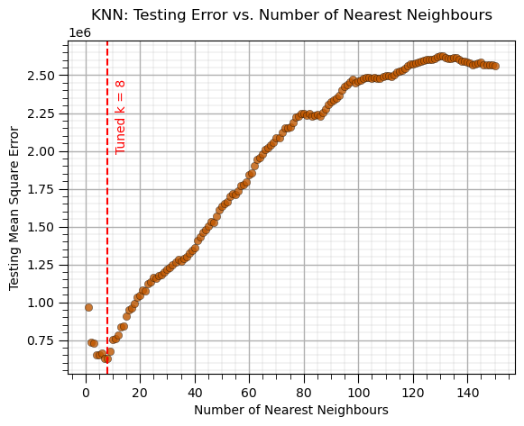
K-Nearest Neighbours (tune)#
Train model parameters on training data with a range of model hyperparameters, select the model hyperparameters with minimum error over the withheld testing data
This requires the following steps,
Loop over the hyperparameter(s) values,
train the model with the retained training data
predict at the withheld testing data
calculate the testing error
Select the hyperparameter that minimized the testing error
k = 1; weights = 'uniform'                                    # set initial, lowest k hyperparameter
MSE_knn_list = []; k_list = []                                # make lists to store the results
while k <= 150:                                               # loop over the k hyperparameter
    knn_model = KNeighborsRegressor(weights = weights, n_neighbors=k, p = 2).fit(X_train,y_train) # instandiate and train the model
    y_test_hat = knn_model.predict(X_test)                    # predict over the testing cases
    MSE = metrics.mean_squared_error(y_test,y_test_hat)       # calculate the MSE testing
    MSE_knn_list.append(MSE)                                  # add to the list of MSE
    k_list.append(k)                                          # append k to an array for plotting
    k = k + 1

tuned_k = k_list[np.argmin(MSE_knn_list)]                     # get the k that minimizes the testing MSE

plt.subplot(111)                                              # plot the testing error vs. hyperparameter
plt.scatter(k_list,MSE_knn_list,s=None, c=utcolor, alpha=0.8, linewidths=0.3, edgecolors="black")
plt.axvline(x=tuned_k, color='red', linestyle='--'); plt.annotate('Tuned k = ' + str(tuned_k),[tuned_k+3,2.0e6],color='red',rotation= 90)
plt.title('KNN: Testing Error vs. Number of Nearest Neighbours'); plt.xlabel('Number of Nearest Neighbours'); plt.ylabel('Testing Mean Square Error')
add_grid()
Linear Regression Model (model parameters)#
Retreive the model parameters.
coef_df = pd.DataFrame({'Feature': ['Intercept'] + list(X.columns),'Coefficient': list(linear_model.intercept_) + list(linear_model.coef_.ravel())})
coef_df
| Feature | Coefficient | |
|---|---|---|
| 0 | Intercept | -4053.511325 |
| 1 | Por | 453.607135 |
| 2 | Perm | 24.707076 |
| 3 | AI | -154.448203 |
| 4 | Brittle | 11.173989 |
| 5 | TOC | -183.938586 |
| 6 | VR | 580.078458 |
Linear Regression Model (prediction test)#
y_test_temp = y_test.copy(deep=True)                          # make a deep copy of the y test DataFrame
y_test_temp['Estimated Prod'] = linear_model.predict(X_test)  # predict over the training data
y_test_temp.head()
| Prod | Estimated Prod | |
|---|---|---|
| 179 | 656.507448 | 379.818856 |
| 155 | 3110.245382 | 2943.388125 |
| 23 | 2581.359826 | 1372.426014 |
| 159 | 6498.151446 | 5563.914978 |
| 96 | 4148.822923 | 4987.375301 |
Linear Regression Model (prediction train)#
y_train_temp = y_train.copy(deep=True)                        # make a deep copy of the y train DataFrame
y_train_temp['Estimated Prod'] = linear_model.predict(X_train)# predict over the training data
y_train_temp.head()
| Prod | Estimated Prod | |
|---|---|---|
| 125 | 3750.106623 | 3938.246048 |
| 68 | 4644.717576 | 3824.308392 |
| 69 | 1991.991593 | 2906.015510 |
| 108 | 6688.360827 | 6653.961261 |
| 131 | 5076.638358 | 5048.864286 |
Linear Regression Model (train)#
Train model parameters on training data, no hyperparameters
linear_model = LinearRegression().fit(X_train,y_train)        # instantiate and train linear regression model, no hyperparmeters
coef_df = pd.DataFrame({'Feature': ['Intercept'] + list(X.columns),'Coefficient': list(linear_model.intercept_) + list(linear_model.coef_.ravel())})
coef_df
| Feature | Coefficient | |
|---|---|---|
| 0 | Intercept | -4053.511325 |
| 1 | Por | 453.607135 |
| 2 | Perm | 24.707076 |
| 3 | AI | -154.448203 |
| 4 | Brittle | 11.173989 |
| 5 | TOC | -183.938586 |
| 6 | VR | 580.078458 |
Listwise Deletion#
Remove all samples that are missing and features.
the “sledge hammer” approach to avoid feature imputation
not recommended, often removes too much data
df_listwise = df_missing.dropna(how='any',inplace=False)      # listwise deletion
df_listwise.describe()
| WellIndex | Por | LogPerm | AI | Brittle | TOC | VR | Production | |
|---|---|---|---|---|---|---|---|---|
| count | 210.000000 | 210.000000 | 210.000000 | 210.000000 | 210.000000 | 210.000000 | 210.000000 | 210.000000 |
| mean | 485.680952 | 14.976381 | 1.407238 | 2.999857 | 49.406143 | 1.005524 | 2.001524 | 2373.025529 |
| std | 292.292307 | 3.072786 | 0.422033 | 0.584267 | 14.311860 | 0.521783 | 0.306854 | 1661.542253 |
| min | 3.000000 | 6.480000 | 0.360000 | 1.330000 | 17.200000 | -0.230000 | 0.900000 | 75.215188 |
| 25% | 206.250000 | 12.682500 | 1.110000 | 2.612500 | 39.117500 | 0.640000 | 1.800000 | 1154.774039 |
| 50% | 477.500000 | 15.035000 | 1.415000 | 3.055000 | 48.320000 | 0.980000 | 2.010000 | 2029.697410 |
| 75% | 729.500000 | 17.085000 | 1.680000 | 3.360000 | 58.547500 | 1.347500 | 2.220000 | 3223.502405 |
| max | 1000.000000 | 24.650000 | 2.480000 | 4.500000 | 86.800000 | 2.560000 | 2.820000 | 12568.644130 |
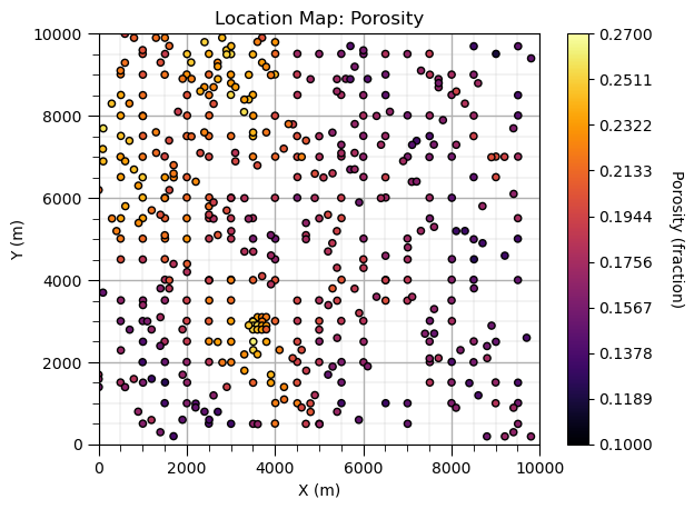
Location Map#
For plotting sparsely sampled features with X and Y sample locations to inspect the spatial structures.
xmin=0; xmax=10000; ymin=0; ymax=10000; vmin=0.1; vmax=0.27   # set plot limits and feature limits
sc = plt.scatter(df_spatial['X'],df_spatial['Y'],c=df_spatial['Porosity'],s=20,edgecolor='black',vmin=vmin,vmax=vmax,cmap = cmap)
cbar = plt.colorbar(sc, orientation="vertical", ticks=np.linspace(vmin,vmax,10)); plt.xlabel('X (m)'); plt.ylabel('Y (m)')
cbar.set_label(r'Porosity (fraction)', rotation=270, labelpad=20); plt.xlim(0,10000); plt.ylim(0,10000); add_grid()
plt.title('Location Map: Porosity'); plt.show()
Mean (imputation)#
A very simple approach for feature imputation, replace the missing values with the mean of the feature,
does on introduce a bias in the mean, but will introduce a bias in the standard deviation and variance
will likely bias low the between predictor and response feature correlation
mean_imputer = SimpleImputer(strategy='mean')                 # instantiate mean imputor
X_imputed = mean_imputer.fit_transform(X_missing)             # train and apply MICE to impute the missing data
X_imputed = pd.DataFrame(X_imputed, columns=X_missing.columns,index=X_missing.index) # make imputed results into a DataFrame with same columns as X
X_imputed.describe()                                          # preview the DataFrame
| Por | LogPerm | AI | Brittle | TOC | VR | |
|---|---|---|---|---|---|---|
| count | 1000.000000 | 1000.000000 | 1000.000000 | 1000.000000 | 1000.000000 | 1000.000000 |
| mean | 14.898708 | 1.383061 | 2.984200 | 49.607696 | 0.999551 | 1.996173 |
| std | 2.933199 | 0.344835 | 0.544243 | 12.532978 | 0.431517 | 0.265394 |
| min | 5.400000 | 0.120000 | 0.960000 | -1.500000 | -0.250000 | 0.900000 |
| 25% | 12.940000 | 1.217500 | 2.630000 | 43.937500 | 0.800000 | 1.897500 |
| 50% | 14.898708 | 1.383061 | 2.984200 | 49.607696 | 0.999551 | 1.996173 |
| 75% | 16.840000 | 1.530000 | 3.302500 | 55.515000 | 1.210000 | 2.110000 |
| max | 24.650000 | 2.580000 | 4.700000 | 93.470000 | 2.710000 | 2.900000 |
Minimum and Maximum (dataframe)#
print('Dataframe Minimum:'); print(df.min())                  # using pandas DataFrame's min and max member functions
print('\nDataframe Maximum:'); print(df.max())
Dataframe Minimum:
Well         1.000000
Por          6.550000
Perm         1.130000
AI           1.280000
Brittle     10.940000
TOC         -0.190000
VR           0.930000
Prod       463.579973
dtype: float64

Dataframe Maximum:
Well        200.000000
Por          23.550000
Perm          9.870000
AI            4.630000
Brittle      84.330000
TOC           2.180000
VR            2.870000
Prod       8428.187903
dtype: float64
Minimum and Maximum (ndarray)#
print('2D ndarray Minimum:'); print(np.min(ndarray_2D))       # using NumPy's min and max functions that flatten internally
print('\n2D ndarray Maximum:'); print(np.max(ndarray_2D))
2D ndarray Minimum:
1516.949331702811

2D ndarray Maximum:
6735.039007281679
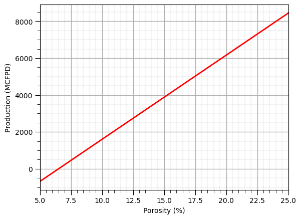
Model Plot (linear 1D)#
We use the follow steps,
make an array of equally spaced values of the predictor feature(s)
predict at all of these predictor values
cross plot the predictions with the predictor values
x_values = np.linspace(5,25,100).reshape(-1,1)                # array of equally space values in the predictor feature
y_hat_linear_1pred = linear_1pred_model.predict(x_values)     # predict over the predictor feature values
plt.plot(np.linspace(5,25,100),y_hat_linear_1pred,color='red',lw=2) # plot the predictions vs. the predictor values
plt.xlabel('Porosity (%)'); plt.ylabel('Production (MCFPD)'); add_grid(); plt.xlim(5,25); plt.show()
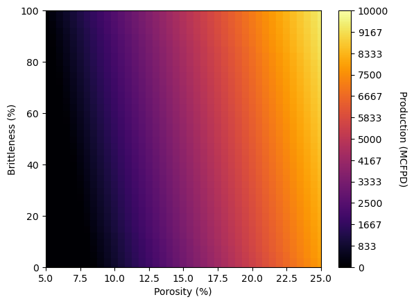
Model Plot (linear 2D)#
We use the follow steps,
make a mesh array of equally spaced values of the predictor feature(s)
predict at all of these predictor values
flatten all meshes to 1D
plot with a colored scatter plot with square markers (s) scalled to fill in the plot
I prefer this method because plt.imshow often is inconsistent with other plots when added as a subplot
XX1, XX2 = np.meshgrid(np.arange(5,25.5,0.5),np.arange(0,102.5,2.5)) # get a regular grid of response feature values
y_hat = linear_2pred_model.predict(np.c_[XX1.ravel(), XX2.ravel()]).reshape(-1)   # predict over grid and convert to a 1D vector
sc = plt.scatter(XX1.ravel(),XX2.ravel(),c=y_hat,marker='s',s=50,vmin=0,vmax=10000,cmap=cmap) # convert XX1/2 to 1D vectors use for scatter plot
cbar = plt.colorbar(sc, orientation="vertical", ticks=np.linspace(0, 10000, 13)); cbar.set_label(r'Production (MCFPD)', rotation=270, labelpad=20)
plt.xlabel('Porosity (%)'); plt.ylabel('Brittleness (%)'); plt.xlim(5,25); plt.ylim(0,100); plt.show()
Model Mean Absolute Error (testing)#
MSE_test = metrics.mean_absolute_error(y_test,y_hat_test)     # calculate the training MSE
print('Model Training MAE: ' + str(MSE_test))                 # print the training MSE
Model Training MAE: 679.7220485741077
Model Mean Absolute Error (training)#
MSE_train = metrics.mean_absolute_error(y_train,y_hat_train)  # calculate the training MSE
print('Model Training MAE: ' + str(MSE_train))                # print the training MSE
Model Training MAE: 713.4026730760603
Model MSE (testing)#
MSE_test = metrics.mean_squared_error(y_test,y_hat_test)      # calculate the training MSE
print('Model Training MSE: ' + str(MSE_test))                 # print the training MSE
Model Training MSE: 731861.1594257785
Model MSE (training)#
MSE_train = metrics.mean_squared_error(y_train,y_hat_train)   # calculate the training MSE
print('Model Training MSE: ' + str(MSE_train))                # print the training MSE
Model Training MSE: 805986.6842431575
Multiple Imputation by Chained Equations#
Feature imputation by iterative application of K-nearest neighbours,
accomplished by multiple passes, the structure in the data is learned to improve the imputation
robust with significant porportion of missing feature values
mice_imputer = IterativeImputer(random_state = seed,max_iter=100) # instantiate Multiple Imputation by Chained Equations (MICE) imputer
X_imputed = mice_imputer.fit_transform(X_missing)             # train and apply MICE to impute the missing data
X_imputed = pd.DataFrame(X_imputed, columns=X_missing.columns,index=X_missing.index) # make imputed results into a DataFrame with same columns as X
X_imputed.describe()                                          # preview the DataFrame
| Por | LogPerm | AI | Brittle | TOC | VR | |
|---|---|---|---|---|---|---|
| count | 1000.000000 | 1000.000000 | 1000.000000 | 1000.000000 | 1000.000000 | 1000.000000 |
| mean | 14.944723 | 1.404668 | 2.980626 | 49.817322 | 1.005436 | 1.990035 |
| std | 3.030406 | 0.397241 | 0.565985 | 14.029791 | 0.492149 | 0.302019 |
| min | 5.400000 | 0.120000 | 0.960000 | -5.422936 | -0.306453 | 0.900000 |
| 25% | 12.850000 | 1.142772 | 2.580000 | 41.384356 | 0.660000 | 1.810000 |
| 50% | 14.950000 | 1.395805 | 3.010000 | 50.077539 | 1.010000 | 1.985885 |
| 75% | 17.052500 | 1.670000 | 3.350314 | 57.951806 | 1.358028 | 2.170000 |
| max | 24.650000 | 2.580000 | 4.700000 | 100.043660 | 2.710000 | 2.927459 |
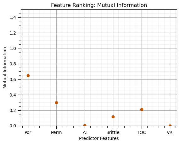
Mutual Information#
Measure of information shared between predictors and the response feature,
robust in the presence of nonlinearity and heteroscedasticity,
MI Value Range |
Interpretation |
|---|---|
Close to 0 |
Variables are nearly independent |
Low (small positive) |
Weak dependency or little shared information |
Moderate |
Some meaningful dependency |
High |
Strong dependency; variables share substantial information |
Very High |
Near deterministic relationship |
mi = mutual_info_regression(X, y.values.ravel(),random_state=0) # calculuate mutual information
mi_series = pd.Series(mi, index=X.columns)                    # convert ndarray to pandas series (column of a DataFrame) for ease of plotting
mi_series.plot(color=utcolor,style='o');
plt.xlabel('Predictor Features'); plt.ylabel('Mutual Information'); plt.ylim(0,1.5); plt.title('Feature Ranking: Mutual Information')
add_grid(); plt.show()
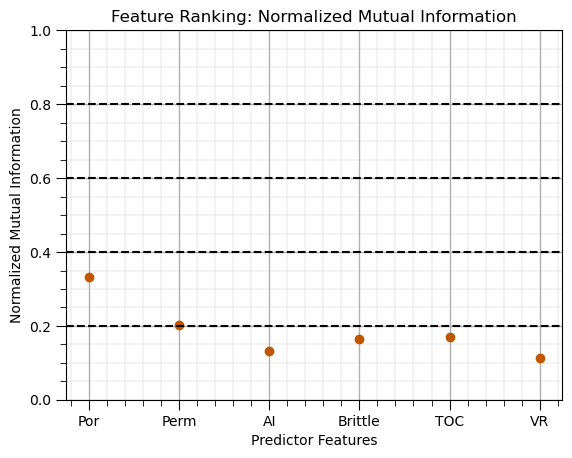
Mutual Information (normalized)#
Measure of information shared between predictors and the response feature,
robust in the presence of nonlinearity and heteroscedasticity
normalized by marginal entropies to have a maximum value of 1.0, 0.0 = no information, 1.0 = perfect information
Here’s the common rule of thumb to assist with interpretation,
NMI Value Range |
Interpretation |
|---|---|
0.0 – 0.2 |
Very weak or negligible relation |
0.2 – 0.4 |
Weak relation |
0.4 – 0.6 |
Moderate relation |
0.6 – 0.8 |
Strong relation |
0.8 – 1.0 |
Very strong or near perfect |
kbd = KBinsDiscretizer(n_bins=10, encode='ordinal', strategy='quantile') # instantiate dicretizer
X_binned = pd.DataFrame(kbd.fit_transform(X), columns=X.columns) # discretize the predictor features
y_bins = pd.qcut(y.values.ravel(), q=10, labels=False, duplicates='drop') # discretize the response features
nmi_scores = []
for col in X_binned.columns:                                  # loop over predictor features
    nmi = normalized_mutual_info_score(X_binned[col], y_bins) # calculate normalize mutual information
    nmi_scores.append(nmi)
nmi_series = pd.Series(nmi_scores, index=X.columns)
nmi_series.plot(color=utcolor,style='o'); plt.xlabel('Predictor Features'); plt.ylabel('Normalized Mutual Information'); plt.ylim(0,1)
plt.title('Feature Ranking: Normalized Mutual Information')
for yvalue in np.arange(0.2,1.0,0.2):
    plt.axhline(y=yvalue, color='black', linestyle='--')      # add interpretation lines
add_grid(); plt.show()
Normalize Predictor Features#
Normalize the predictor features to remove any sensitivity to feature range or variance, for example,
put features all on equal playing field for distance calculations
Min / max normalization forces the minimum to be 0.0 and the maximum to be 1.0
normalizer = MinMaxScaler()                                   # instantiate min / max normalizer
norm_array = normalizer.fit_transform(X)                      # normalize the predictor features
X_norm = pd.DataFrame(norm_array, columns=X.columns)          # convert output to a DataFrame
X_norm.describe()                                             # preview the DataFrame
| Por | Perm | AI | Brittle | TOC | VR | |
|---|---|---|---|---|---|---|
| count | 200.000000 | 200.000000 | 200.000000 | 200.000000 | 200.000000 | 200.000000 |
| mean | 0.496538 | 0.366219 | 0.504134 | 0.507180 | 0.498080 | 0.533144 |
| std | 0.174775 | 0.198057 | 0.169220 | 0.192526 | 0.203202 | 0.155066 |
| min | 0.000000 | 0.000000 | 0.000000 | 0.000000 | 0.000000 | 0.000000 |
| 25% | 0.374265 | 0.227975 | 0.378358 | 0.365377 | 0.340717 | 0.432990 |
| 50% | 0.501176 | 0.332380 | 0.500000 | 0.525548 | 0.514768 | 0.530928 |
| 75% | 0.638382 | 0.475686 | 0.616418 | 0.644809 | 0.649789 | 0.625000 |
| max | 1.000000 | 1.000000 | 1.000000 | 1.000000 | 1.000000 | 1.000000 |
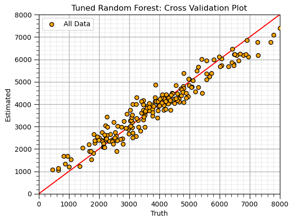
Random Forest (retrain tuned model)#
Apply tuned hyperparameters and retrain the model.
this is the model that we will use for future predictions, real-world use
max_leaf_node_tuned = 40; num_tree = 20; max_features = 2                # random forest model hyperparameters
random_forest = RandomForestRegressor(max_leaf_nodes=max_leaf_node_tuned,random_state=seed,n_estimators=num_tree,max_features=max_features,
                                       oob_score=True,bootstrap=True)
random_forest.fit(X,y.values.ravel())
y_rf_hat = random_forest.predict(X)                      # predict over the testing cases
plt.scatter(y,y_rf_hat,color='orange',edgecolor='black',label=r'All Data',zorder=10) # scatter plot
plt.ylabel('Estimated'); plt.xlabel('Truth'); plt.title('Tuned Random Forest: Cross Validation Plot'); plt.legend(loc = 'upper left')
plt.plot([0,8000],[0,8000],color='red'); plt.xlim(0,8000,); plt.ylim(0,8000)
add_grid()
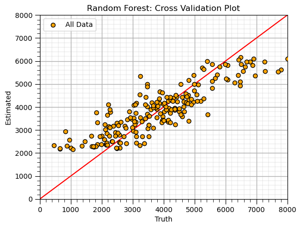
Random Forest (train)#
max_leaf_node = 5; num_tree = 20; max_features = 2                # random forest model hyperparameters
random_forest = RandomForestRegressor(max_leaf_nodes=max_leaf_node,random_state=seed,n_estimators=num_tree,max_features=max_features,
                                       oob_score=True,bootstrap=True)
random_forest.fit(X,y.values.ravel())
y_rf_hat = random_forest.predict(X)                      # predict over the testing cases
plt.scatter(y,y_rf_hat,color='orange',edgecolor='black',label=r'All Data',zorder=10) # scatter plot
plt.ylabel('Estimated'); plt.xlabel('Truth'); plt.title('Random Forest: Cross Validation Plot'); plt.legend(loc = 'upper left')
plt.plot([0,8000],[0,8000],color='red'); plt.xlim(0,8000,); plt.ylim(0,8000)
add_grid()
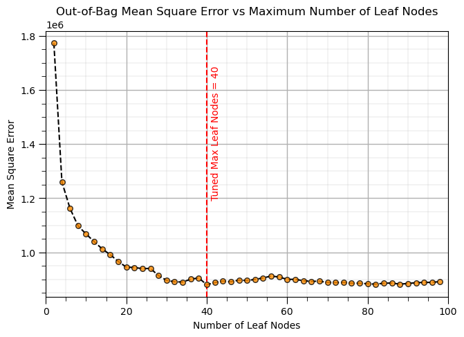
Random Forest (tune)#
max_leaf_node_mat = np.arange(2,100,2)                        # set the random forest hyperparameters
max_features = 1
trained_forests = []
MSE_oob_list = []; node_list = []

index = 1
for max_leaf_node in max_leaf_node_mat:                       # loop over number of trees in our random forest
    trained_forest = RandomForestRegressor(max_leaf_nodes=max_leaf_node, random_state=seed,n_estimators=num_tree,
            oob_score = True,bootstrap=True,max_features=max_features).fit(X = X, y = y.values.ravel())
    trained_forests.append(trained_forest)
    oob_y_hat = trained_forest.oob_prediction_
    oob_y = y[oob_y_hat > 0.0]; oob_y_hat = oob_y_hat[oob_y_hat > 0.0]; # remove if not estimated
    MSE_oob_list.append(metrics.mean_squared_error(oob_y,oob_y_hat)); node_list.append(max_leaf_node)
    index = index + 1

tuned_node = node_list[np.argmin(MSE_oob_list)]               # get the k that minimizes the testing MSE

plt.subplot(121)
plt.scatter(node_list,MSE_oob_list,color='darkorange',edgecolor='black',alpha=0.8,s=30,zorder=10)
plt.plot(node_list,MSE_oob_list,color='black',ls='--',zorder=1)
plt.axvline(x=tuned_node, color='red', linestyle='--')
plt.annotate('Tuned Max Leaf Nodes = ' + str(tuned_node),[tuned_node+1,1.2e6],color='red',rotation= 90)
plt.xlabel('Number of Leaf Nodes'); plt.ylabel('Mean Square Error')
plt.title('Out-of-Bag Mean Square Error vs Maximum Number of Leaf Nodes')
add_grid(); plt.xlim(0,100)
plt.subplots_adjust(left=0.0, bottom=0.0, right=2.0, top=0.8, wspace=0.2, hspace=0.2); plt.show()
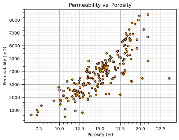
Scatter Plot#
plt.scatter(X['Por'],y['Prod'],color='darkorange',edgecolor='black',s=20); plt.xlabel('Porosity (%)'); plt.ylabel('Permeability (mD)')
add_grid(); plt.title('Permeability vs. Porosity'); plt.show();
Standardize Predictor Features#
Standardize the predictor features to remove any sensitivity to feature range or variance, for example,
put features all on equal playing field for distance calculations
Standardization forces the mean to be 0.0 and the standard deviation to be 1.0
scaler = StandardScaler()                                     # instantiate standardizer
standard_array = scaler.fit_transform(X)                      # standardize the predictor features
X_stand = pd.DataFrame(standard_array, columns=X.columns)     # convert output to a DataFrame
X_stand.describe()                                            # preview the DataFrame
| Por | Perm | AI | Brittle | TOC | VR | |
|---|---|---|---|---|---|---|
| count | 2.000000e+02 | 2.000000e+02 | 2.000000e+02 | 2.000000e+02 | 2.000000e+02 | 2.000000e+02 |
| mean | 2.486900e-16 | -6.217249e-17 | 4.130030e-16 | 2.042810e-16 | 3.375078e-16 | 9.081624e-16 |
| std | 1.002509e+00 | 1.002509e+00 | 1.002509e+00 | 1.002509e+00 | 1.002509e+00 | 1.002509e+00 |
| min | -2.848142e+00 | -1.853701e+00 | -2.986650e+00 | -2.640962e+00 | -2.457313e+00 | -3.446814e+00 |
| 25% | -7.013606e-01 | -6.997528e-01 | -7.451372e-01 | -7.383912e-01 | -7.763606e-01 | -6.475066e-01 |
| 50% | 2.660490e-02 | -1.712823e-01 | -2.449306e-02 | 9.564649e-02 | 8.233024e-02 | -1.432979e-02 |
| 75% | 8.136175e-01 | 5.540977e-01 | 6.652032e-01 | 7.166516e-01 | 7.484661e-01 | 5.938532e-01 |
| max | 2.887855e+00 | 3.208033e+00 | 2.937664e+00 | 2.566186e+00 | 2.476256e+00 | 3.018254e+00 |
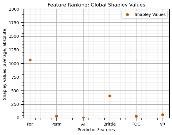
Shapley Values (feature ranking)#
max_leaf_nodes = 20
tree_shap_model = DecisionTreeRegressor(max_leaf_nodes = max_leaf_nodes).fit(X, y)
explainer = shap.Explainer(tree_shap_model, X)                          # Explain the model with SHAP
shap_values = explainer.shap_values(X)
shap_avg = np.average(np.abs(shap_values),axis = 0)
shap_df = pd.DataFrame({'Feature': list(X.columns),'Shapley Values': list(shap_avg)}); shap_df.set_index('Feature',inplace=True)
shap_df.plot(color=utcolor,style='o'); plt.xlabel('Predictor Features'); plt.ylabel('Shapley Values (average, absolute)'); plt.ylim(0,2000)
plt.title('Feature Ranking: Global Shapley Values'); add_grid(); plt.show()
Summary Statistics (DataFrame)#
df.describe() # calculate the summary statistics of each feature
| Well | Por | Perm | AI | Brittle | TOC | VR | Prod | |
|---|---|---|---|---|---|---|---|---|
| count | 200.000000 | 200.000000 | 200.000000 | 200.000000 | 200.000000 | 200.000000 | 200.000000 | 200.000000 |
| mean | 100.500000 | 14.991150 | 4.330750 | 2.968850 | 48.161950 | 0.990450 | 1.964300 | 3874.056957 |
| std | 57.879185 | 2.971176 | 1.731014 | 0.566885 | 14.129455 | 0.481588 | 0.300827 | 1615.551334 |
| min | 1.000000 | 6.550000 | 1.130000 | 1.280000 | 10.940000 | -0.190000 | 0.930000 | 463.579973 |
| 25% | 50.750000 | 12.912500 | 3.122500 | 2.547500 | 37.755000 | 0.617500 | 1.770000 | 2616.522434 |
| 50% | 100.500000 | 15.070000 | 4.035000 | 2.955000 | 49.510000 | 1.030000 | 1.960000 | 3801.156899 |
| 75% | 150.250000 | 17.402500 | 5.287500 | 3.345000 | 58.262500 | 1.350000 | 2.142500 | 4786.375831 |
| max | 200.000000 | 23.550000 | 9.870000 | 4.630000 | 84.330000 | 2.180000 | 2.870000 | 8428.187903 |
Train and Test Split#
Random splitting of the data into train and test splits.
test_proportion = 0.2                                         # set the proportion of withheld testing data
X_train, X_test, y_train, y_test = train_test_split(X, y, test_size=test_proportion, random_state=seed) # train and test split
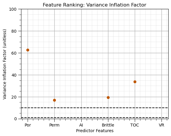
Variance Inflation Factor#
Feature ranking method that only considers the linear redundancy between the predictor features,
relationship with the response feature, relevancy is not considered
general used as a screening method to remove features before more comprehensive feature ranking
vif_data = pd.Series(                                         # loop over predictor features and store result in pandas series for ease of plotting
    [variance_inflation_factor(X.values, i) for i in range(X.values.shape[1])],
    index=X.columns)
vif_data.plot(color=utcolor,style='o'); plt.xlabel('Predictor Features'); plt.ylabel('Variance Inflation Factor (unitless)'); plt.ylim(0,100)
plt.axhline(y=1, color='black', linestyle='--'); plt.axhline(y=10, color='black', linestyle='--');
add_grid(); plt.title('Feature Ranking: Variance Inflation Factor'); plt.show()
About the Author#

Michael Pyrcz is a professor in the Cockrell School of Engineering, and the Jackson School of Geosciences, at The University of Texas at Austin, where he researches and teaches subsurface, spatial data analytics, geostatistics, and machine learning. Michael is also,
the principal investigator of the Energy Analytics freshmen research initiative and a core faculty in the Machine Learn Laboratory in the College of Natural Sciences, The University of Texas at Austin
an associate editor for Computers and Geosciences, and a board member for Mathematical Geosciences, the International Association for Mathematical Geosciences.
Michael has written over 70 peer-reviewed publications, a Python package for spatial data analytics, co-authored a textbook on spatial data analytics, Geostatistical Reservoir Modeling and author of two recently released e-books, Applied Geostatistics in Python: a Hands-on Guide with GeostatsPy and Applied Machine Learning in Python: a Hands-on Guide with Code.
All of Michael’s university lectures are available on his YouTube Channel with links to 100s of Python interactive dashboards and well-documented workflows in over 40 repositories on his GitHub account, to support any interested students and working professionals with evergreen content. To find out more about Michael’s work and shared educational resources visit his Website.
Want to Work Together?#
I hope this content is helpful to those that want to learn more about subsurface modeling, data analytics and machine learning. Students and working professionals are welcome to participate.
Want to invite me to visit your company for training, mentoring, project review, workflow design and / or consulting? I’d be happy to drop by and work with you!
Interested in partnering, supporting my graduate student research or my Subsurface Data Analytics and Machine Learning consortium (co-PI is Professor John Foster)? My research combines data analytics, stochastic modeling and machine learning theory with practice to develop novel methods and workflows to add value. We are solving challenging subsurface problems!
I can be reached at mpyrcz@austin.utexas.edu.
I’m always happy to discuss,
Michael
Michael Pyrcz, Ph.D., P.Eng. Professor, Cockrell School of Engineering and The Jackson School of Geosciences, The University of Texas at Austin
More Resources Available at: Twitter | GitHub | Website | GoogleScholar | Geostatistics Book | YouTube | Applied Geostats in Python e-book | Applied Machine Learning in Python e-book | LinkedIn
Comments#
These are some basic code snipets for predictive machine learning in Python. Much more could be done and discussed, I have many more resources. Check out my shared resource inventory and the YouTube lecture links at the start of this chapter with resource links in the videos’ descriptions.
I hope this is helpful,
Michael