Predictive Machine Learning with scikit-learn

Predictive Machine Learning with scikit-learn#

Michael J. Pyrcz, Professor, The University of Texas at Austin

Chapter of e-book “Applied Machine Learning in Python: a Hands-on Guide with Code”.

Cite this e-Book as:

Pyrcz, M.J., 2024, Applied Machine Learning in Python: A Hands-on Guide with Code [e-book]. Zenodo. doi:10.5281/zenodo.15169138

The workflows in this book and more are available here:

Cite the MachineLearningDemos GitHub Repository as:

Pyrcz, M.J., 2024, MachineLearningDemos: Python Machine Learning Demonstration Workflows Repository (0.0.3) [Software]. Zenodo. DOI: 10.5281/zenodo.13835312. GitHub repository: GeostatsGuy/MachineLearningDemos

By Michael J. Pyrcz
© Copyright 2025.

This chapter is a tutorial for / demonstration of Predictive Machine Learning with scikit-learn.

YouTube Lecture: check out my lectures on:

These lectures are all part of my Machine Learning Course on YouTube with linked well-documented Python workflows and interactive dashboards. My goal is to share accessible, actionable, and repeatable educational content. If you want to know about my motivation, check out Michael’s Story.

Motivation for Predictive Machine Learning with scikit-learn#

This chapter is unusual for me. As a professor, I avoid lectures that focus on the specific tools, as I would rather teach the principles and then introduce the examples with the common tools. It is my opinion that,

theory will outlast any available software tools
without a theory focus I may encourage black-box model use
with a strong understanding of the theory, one could pick up any software as needed

But in this case,

scikit-learn is such a common machine learning package for machine learning that is very widely used
throughout this e-book I use scikit-learn
scikit-learn uses a nuts and bolts approach to build machine learning workflows that maximizes flexibility
scikit-learn provides the theory in the docs or links to original publications

In summary, scikit-learn get me and I see the package as a partner in education! Thank you!

So I have decided to add this chapter focused on the methods for machine learning modeling with scikit-learn.

Machine Learning-based Prediction#

Here’s a simple workflow, demonstration of scikit-learn training and tuning a machine learning model with a simple dataset.

I provide this as the most basic, minimum Python workflow to assist those learning predictive machine learning
I demonstration model training and tuning (by-hand and automatically), including the pipeline approach
Given the 1 predictor feature and 1 response for ease of data and model visualization

This provides an opportunity to run and visualize a variety of machine learning models for experiential learning.

Machine Learning-based Prediction#

We build a decision tree-based predictive machine learning models with supervised learning:

Prediction

non-parametric method for regression (continuous response) and classification (categorical response)
a function \(\hat{f}\) of the nearest \(k\) training data in predictor feature space such that we predict a response feature \(Y\) from a set of predictor features \(X_1,\ldots,X_m\).
the prediction is of the form:

\begin{equation} \hat{Y} = \hat{f}(X_1,\ldots,X_m) + \epsilon \end{equation}

where \(\epsilon\) is an error term.

Supervised Learning

the response feature, \(Y\), is available over the training and testing data

Load the Required Libraries#

The following code loads the required libraries. These should have been installed with Anaconda 3.

ignore_warnings = True                                        # ignore warnings?
import os                                                     # to set current working directory 
import pandas as pd                                           # DataFrames and plotting
import numpy as np                                            # arrays and matrix math
import matplotlib.pyplot as plt                               # plotting
from matplotlib.ticker import (MultipleLocator, AutoMinorLocator) # control of axes ticks
from sklearn import metrics                                   # measures to check our models
from sklearn.model_selection import train_test_split          # random train and test data split
from sklearn import tree                                      # tree program from scikit learn (package for machine learning)
plt.rc('axes', axisbelow=True)                                # plot all grids below the plot elements
if ignore_warnings == True:                                   
    import warnings
    warnings.filterwarnings('ignore')
cmap = plt.cm.inferno                                         # color map
seed = 42                                                     # random number seed

If you get a package import error, you may have to first install some of these packages. This can usually be accomplished by opening up a command window on Windows and then typing ‘python -m pip install [package-name]’. More assistance is available with the respective package docs.

Set the Random Number Seed#

These workflows and models may use random processes, e.g.:

random train and test split with cross validation and k-fold cross validation
random selection of a subset of features to consider for the next split

np.random.seed(seed)                                        # scikit-learn uses the NumPy seed

Declare functions#

Let’s define a function for plotting gridlines.

def add_grid():
    plt.gca().grid(True, which='major',linewidth = 1.0); plt.gca().grid(True, which='minor',linewidth = 0.2) # add y grids
    plt.gca().tick_params(which='major',length=7); plt.gca().tick_params(which='minor', length=4)
    plt.gca().xaxis.set_minor_locator(AutoMinorLocator()); plt.gca().yaxis.set_minor_locator(AutoMinorLocator()) # turn on minor ticks   

Set the working directory#

I always like to do this so I don’t lose files and to simplify subsequent read and writes (avoid including the full address each time).

# not needed currently
#os.chdir("c:/PGE383")                                       # set the working directory

You will have to update the part in quotes with your own working directory and the format is different on a Mac (e.g. “~/PGE”).

Read the data table#

We use a data “1D_Porosity.csv” comma delimited file from my GitHub GeoDataSets Respository.

this code loads the data directly from my GitHub repository.
if you have the data file available locally (i.e. you are not connected to the internet) set the working directory to the location with the data file and use the second line below

my_data = pd.read_csv("https://raw.githubusercontent.com/GeostatsGuy/GeoDataSets/master/1D_Porosity.csv") # load the comma delimited data file
#my_data = pd.read_csv("1D_Porosity.csv")                     # load the comma delimited data file locally
X = pd.DataFrame(data = my_data.loc[:,'Depth'])               # ensure X and y features are DataFrames
y = pd.DataFrame(data = my_data.loc[:,'Nporosity'])
X.head(n=2); y.head(n=2)                                      # preview the predictor feature
print('Loaded ' + str(len(my_data)) + ' samples, with features = ' + str(my_data.columns.values) + '.')

Loaded 40 samples, with features = ['Depth' 'Nporosity'].

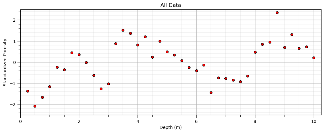
Plot the Available Data#

Let’s do a simple scatter plot to check the data.

plt.scatter(X,y,color='red',s=30,edgecolor='black',alpha=1.0); plt.xlabel('Depth (m)'); plt.ylabel('Standardized Porosity'); plt.title('All Data'); 
plt.xlim([0,10.25]); plt.ylim([-2.5,2.5]); add_grid()
plt.subplots_adjust(left=0.0, bottom=0.0, right=1.5, top=0.7, wspace=0.2, hspace=0.2);

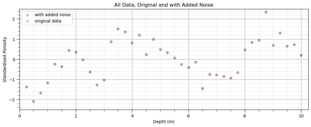
_images/c8f68d96b92a64e674753dd321abb3376a788853f792000775c676b02927aec1.png

Optional: Add Random Error to the Response Feature, \(y\)#

For more experiential learning consider repeating this workflow with different amounts of additional error

to observe issues of model overfit consider adding some additional error,

error_stdev = 0.0                                           # standard deviation of additional random error

error_stdev = 0.0                                             # standard deviation of additional random error
y_orig = y.copy(deep = True)                                  # make a deep copy of original dataset
y['Nporosity'] = y['Nporosity'] + np.random.normal(loc = 0, scale = error_stdev, size = y.shape[0])
plt.scatter(X,y,color='blue',s=30,edgecolor='black',alpha=0.2,label='with added noise'); plt.xlabel('Depth (m)'); 
plt.ylabel('Standardized Porosity'); plt.title('All Data, Original and with Added Noise'); plt.xlim([0,10.25]); plt.ylim([-2.5,2.5])
plt.scatter(X,y_orig,color='red',s=30,edgecolor='black',alpha=0.2,label='original data'); plt.xlabel('Depth (m)'); 
plt.ylabel('Standardized Porosity'); plt.legend(loc='upper left')
plt.xlim([0,10.25]); plt.ylim([-2.5,2.5]); add_grid()
plt.subplots_adjust(left=0.0, bottom=0.0, right=1.5, top=0.7, wspace=0.2, hspace=0.2);

_images/db6bdae8f03df1faab8e473a6c4ac4068bec1a1c0601e89ed59590368330bf1c.png

Fast Forward Through Data Analytics#

This workflow is focussed on building predictive machine learning models

for brevity we skip data checking, data analytics, statistical analysis, feature transformations etc.
we skip all the way to model building
we don’t even discuss model selection, feature selection, nor robust hyperparameter tuning

This is the most simple predictive machine learning workflow possible!

basics for machine learning with scikit-learn in Python. Nothing more.

Let’s Build a Predictive Machine Learning Model#

We use the following steps to build our model

instantiate the machine learning model with hyperparameters
fit, train the machine learing model to the training data
predict, check the trained machine learning models to predict at withheld testing data
select the optimum hyperparameters, hyperparameter tuning
refit the model by training with all data given the tuned hyperparmaeters

We will use the train - test approach, an alternative is the train, validate and test approach.

we will start simple and cover k-fold cross validation and scikit-learn pipeline class later

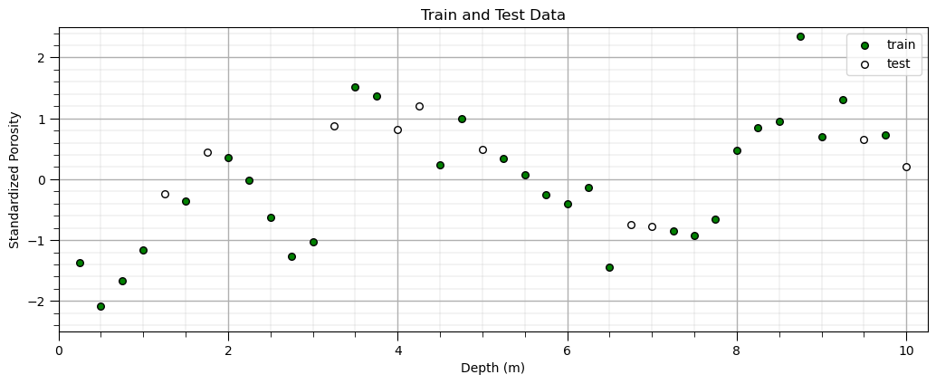
Split Train and Test#

We will demonstrate the following hyperparameter tuning methods:

cross validation - split 25% of data as withheld testing data, only 25% of data are tested
k-fold cross validation - calculate average error over k folds, all data are tested

Let’s start with cross validation and then demonstrate k-fold cross validation.

X_train, X_test, y_train, y_test = train_test_split(X,y, test_size=0.25, random_state=seed) # train and test split
plt.scatter(X_train,y_train,color='green',s=30,edgecolor='black',alpha=1.0,label='train'); plt.xlabel('Depth (m)') 
plt.ylabel('Standardized Porosity'); plt.title('Train and Test Data'); plt.xlim([0,10.25]); plt.ylim([-2.5,2.5]) 
plt.scatter(X_test,y_test,color='white',s=30,edgecolor='black',alpha=1.0,label='test'); plt.xlabel('Depth (m)')
plt.ylabel('Standardized Porosity');plt.legend(loc='upper right'); plt.xlim([0,10.25]); plt.ylim([-2.5,2.5]); add_grid()
plt.subplots_adjust(left=0.0, bottom=0.0, right=1.5, top=0.7, wspace=0.2, hspace=0.2);

_images/8301051d675ae545cbd9a77b7b63baad14810e3e9f3dfd6e299fd5ce3e5cdd5c.png

Build a Decision Tree Model#

Let’s instantiate (set the hyperparameter(s)) and fit (train with training data) a decision tree regression model to our data.

max_leaf_nodes = 6                                            # set the hyperparameter
our_tree = tree.DecisionTreeRegressor(max_leaf_nodes = max_leaf_nodes) # instantiate the model
our_tree = our_tree.fit(X_train, y_train)                     # fit the model to the trainin data

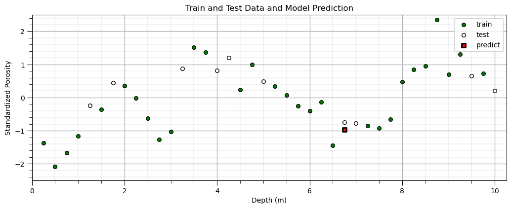
Predict With a Decision Tree Model#

Now let’s make a prediction with our trained decision tree model.

itest = 3; depth = X_test['Depth'].values[itest]            # set the predictor value for our prediction
spor = our_tree.predict([[depth]])                          # predict with our trained model
plt.scatter(X_train,y_train,color='green',s=30,edgecolor='black',alpha=1.0,label='train'); plt.xlabel('Depth (m)'); 
plt.ylabel('Standardized Porosity'); plt.title('Train and Test Data and Model Prediction'); plt.xlim([0,10.25]); plt.ylim([-2.5,2.5]) 
plt.scatter(X_test,y_test,color='white',s=30,edgecolor='black',alpha=1.0,label='test'); plt.xlabel('Depth (m)')
plt.ylabel('Standardized Porosity');plt.legend(loc='upper right')
plt.scatter(depth,spor,color='red',s=30,marker='s',edgecolor='black',alpha=1.0,lw=2,label='predict'); plt.xlabel('Depth (m)') 
plt.ylabel('Standardized Porosity');plt.legend(loc='upper right'); plt.xlim([0,10.25]); plt.ylim([-2.5,2.5]); add_grid()
plt.subplots_adjust(left=0.0, bottom=0.0, right=1.5, top=0.7, wspace=0.2, hspace=0.2); add_grid()

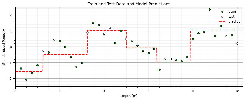
_images/c8659b494469d1cf1349fd8143fe016473544dea1159f62300489b493236734c.png

Predict Over a Range of Predictor Feature Values with a Decision Tree Model#

Now, let’s make predictions over a range of predictor feature values so we can visualize the model.

this is easy to do since we have just 1 predictor feature

depths = np.linspace(0,10.25,1000)                          # set the predictor values for our prediction
spors = our_tree.predict(depths.reshape(-1, 1))             # predict with our trained model
plt.scatter(X_train,y_train,color='green',s=30,edgecolor='black',alpha=1.0,label='train'); plt.xlabel('Depth (m)') 
plt.ylabel('Standardized Porosity'); plt.title('Train and Test Data and Model Predictions'); plt.xlim([0,10.25]); plt.ylim([-2.5,2.5])
plt.scatter(X_test,y_test,color='white',s=30,edgecolor='black',alpha=1.0,label='test'); plt.xlabel('Depth (m)') 
plt.ylabel('Standardized Porosity');plt.legend(loc='upper right')
plt.plot(depths,spors,color='red',alpha=1.0,label='predict',linestyle='--',lw=2,zorder=-1); plt.xlabel('Depth (m)'); plt.ylabel('Standardized Porosity')
plt.xlim([0,10.25]); plt.ylim([-2.5,2.5]); add_grid()
plt.legend(loc='upper right'); plt.subplots_adjust(left=0.0, bottom=0.0, right=1.5, top=0.7, wspace=0.2, hspace=0.2);

_images/3a5c6ea1ec85203a0f15c3d46ae86783757808f467cadc500454f9c887228fe0.png

Changing the Model Hyperparameter(s)#

Let’s try changing the model complexity and refitting the model.

max_leaf_nodes = 10                                         # set the hyperparameter
our_tree = tree.DecisionTreeRegressor(max_leaf_nodes = max_leaf_nodes) # instantiate the model
our_tree = our_tree.fit(X_train, y_train)                   # fit the model to the trainin data
spors = our_tree.predict(depths.reshape(-1, 1))             # predict with our trained model
plt.scatter(X_train,y_train,color='green',s=30,edgecolor='black',alpha=1.0,label='train'); 
plt.xlabel('Depth (m)'); plt.ylabel('Standardized Porosity'); plt.xlim([0,10.25]); plt.ylim([-2.5,2.5]) 
plt.scatter(X_test,y_test,color='white',s=30,edgecolor='black',alpha=1.0,label='test'); plt.xlabel('Depth (m)')
plt.ylabel('Standardized Porosity');plt.legend(loc='upper right')
plt.plot(depths,spors,color='red',alpha=1.0,label='predict',linestyle='--',lw=2); plt.xlabel('Depth (m)'); 
plt.ylabel('Standardized Porosity');plt.legend(loc='upper right'); plt.xlim([0,10.25]); plt.ylim([-2.5,2.5]); add_grid()
plt.subplots_adjust(left=0.0, bottom=0.0, right=1.5, top=0.7, wspace=0.2, hspace=0.2);

_images/d3b73736375ae3ab790c7b21e2c4c20d28ebdffc2556a99912efb733b3fd7d82.png

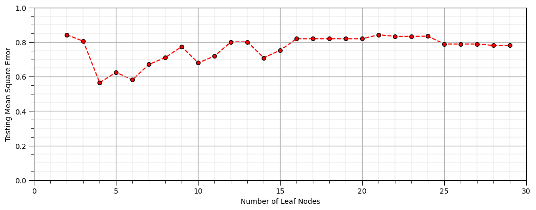
Tuning the Model Hyperparameter(s)#

To tune the model hyperparameters we need a metric to summarize model error over the withheld testing data

let’s predict at the testing data and calculate our metric, testing mean square error.

leaf_nodes = 7                                              # set the hyperparameter
our_tree = tree.DecisionTreeRegressor(max_leaf_nodes = leaf_nodes) # instantiate the model
our_tree = our_tree.fit(X_train, y_train)                   # fit the model to the trainin data
y_predict = our_tree.predict(X_test)                        # predict at the testing data locations
mse = metrics.mean_squared_error(y_test,y_predict)
print('Testing MSE is ' + str(round(mse,2)) + '.')

Testing MSE is 0.67.

and we need to rebuild the model with a variable level of complexity

let’s loop over the number of leaf nodes and plot the performance over the withheld testing data

nodes = []; scores = []; max_leaf_nodes = 30
for i, nnode in enumerate(np.arange(2,max_leaf_nodes,1)):
    our_tree = tree.DecisionTreeRegressor(max_leaf_nodes = nnode).fit(X_train, y_train) # instantiate / fit
    y_predict = our_tree.predict(X_test)                    # predict at the testing data locations
    nodes.append(nnode); scores.append(metrics.mean_squared_error(y_test,y_predict))
plt.scatter(nodes,scores,color='red',s=30,edgecolor='black',alpha=1.0,label='train'); 
plt.plot(nodes,scores,color='red',alpha=1.0,linestyle='--',zorder=-1); plt.xlabel('Depth (m)'); plt.ylabel('Standardized Porosity') 
plt.xlim([1,max_leaf_nodes]); plt.xlabel('Number of Leaf Nodes'); plt.ylabel('Testing Mean Square Error')
plt.xlim([0,max_leaf_nodes]); plt.ylim([0.0,1.0]); add_grid()
plt.subplots_adjust(left=0.0, bottom=0.0, right=1.5, top=0.7, wspace=0.2, hspace=0.2)

_images/d93257b45568bdd5ca8115c16b6ffab50c3eeae024f20178c1f5b9fc272cb45f.png

For a more robust assessment of performance let’s use scikit-learns k-fold cross validation.

from sklearn.model_selection import cross_val_score as kfold       # cross validation methods
nodes = []; scores = []; max_leaf_nodes = 30
for i, nnode in enumerate(np.arange(2,max_leaf_nodes,1,dtype = int)):
    our_tree = tree.DecisionTreeRegressor(max_leaf_nodes = nnode) # instantiate / fit
    nodes.append(nnode); 
    scores.append(abs(kfold(estimator=our_tree,X=X,y=y,cv=4,n_jobs=4,scoring = "neg_mean_squared_error").mean()))
plt.scatter(nodes,scores,color='red',s=30,edgecolor='black',alpha=1.0,label='train')
plt.plot(nodes,scores,color='red',alpha=1.0,linestyle='--'); plt.xlabel('Depth (m)') 
plt.ylabel('Standardized Porosity'); plt.xlim([1,max_leaf_nodes]); plt.xlabel('Number of Leaf Nodes'); plt.ylabel('Testing Mean Square Error')
plt.xlim([0,max_leaf_nodes]); plt.ylim([0.0,4.0]); add_grid()
plt.subplots_adjust(left=0.0, bottom=0.0, right=1.5, top=0.7, wspace=0.2, hspace=0.2)

_images/c0edb899e876f1ebd639ac3d6c4eb5b5a9fe13138c12076aa8086978cb7789bc.png

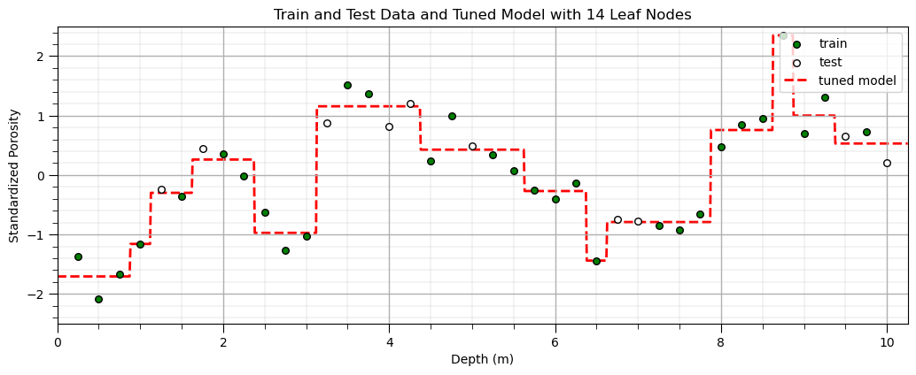
The main product from all of the previous work is the tuned hyperparameter, the optimum model complexity.

now we refit the tuned model, train the model on all the data and our tuned model is ready for real-world use
once again we are assuming a train and test workflow, not a train, validate and test workflow

tuned_nodes = nodes[np.argmin(scores)]
our_tuned_tree = tree.DecisionTreeRegressor(max_leaf_nodes = tuned_nodes).fit(X, y) # instantiate / fit
tuned_spors = our_tuned_tree.predict(depths.reshape(-1, 1))             # predict with our trained model
plt.scatter(X_train,y_train,color='green',s=30,edgecolor='black',alpha=1.0,label='train')
plt.xlabel('Depth (m)'); plt.ylabel('Standardized Porosity')
plt.title('Train and Test Data and Tuned Model with ' + str(tuned_nodes) + ' Leaf Nodes')
plt.xlim([0,10.25]); plt.ylim([-2.5,2.5])
plt.scatter(X_test,y_test,color='white',s=30,edgecolor='black',alpha=1.0,label='test'); 
plt.xlabel('Depth (m)'); plt.ylabel('Standardized Porosity');plt.legend(loc='upper right')
plt.plot(depths,tuned_spors,color='red',alpha=1.0,label='tuned model',linestyle='--',lw=2,zorder=-1); 
plt.xlabel('Depth (m)'); plt.ylabel('Standardized Porosity');plt.legend(loc='upper right'); add_grid()
plt.subplots_adjust(left=0.0, bottom=0.0, right=1.5, top=0.7, wspace=0.2, hspace=0.2);

_images/a69faa8f42377a8d0bc8f93c7f2b21baf60c67eb5e475c3ade5d40904f40b23c.png

Complete Workflow with Pipelines#

Let’s repeat the above workflow with a pipline from scikit-learn. Here some general comments:

pipeline workflow steps - list of steps, custom labels and the associated scikit-learn classes
choices and hyperparameters - as a dictionary with combined step custom labels and hyperparameter names
workflow scenarios - we can specify lists of choices and hyperparameters
consistent iteration - the entire workflow is repeated for the full combinatorial
best model selected - best combination of model hyperparameters and choices are refit with all data

from sklearn.pipeline import Pipeline                       # machine learning modeling pipeline
pipe = Pipeline([                                           # the machine learning workflow as a pipeline object
    ('tree', tree.DecisionTreeRegressor())
])

params = {                                                  # the machine learning workflow method's parameters
    'tree__max_leaf_nodes': np.arange(2,max_leaf_nodes,1,dtype = int)
}

from sklearn.model_selection import GridSearchCV            # model hyperparameter grid search
grid_cv_tuned = GridSearchCV(pipe, params, scoring = 'neg_mean_squared_error', # grid search cross validation 
                             cv=4,refit = True);

grid_cv_tuned.fit(X,y);                                      # fit model with tuned hyperparameters
print('Tuned maximum number of leaf nodes = ' + str(grid_cv_tuned.best_params_['tree__max_leaf_nodes']) + '.')
depth = 2.5
print('Prediction at depth = ' + str(depth) + ' m is ' + str(np.round(grid_cv_tuned.predict([[depth]]),2))) # predict with our trained model) + '.')

Tuned maximum number of leaf nodes = 14.
Prediction at depth = 2.5 m is [-0.97]

Comments#

This was a very simple demonstration of predictive machine learning model building with Python’s scikit-learn.

this is a basic introduction, much more could be done

I hope this was helpful,

Michael

Michael Pyrcz, Ph.D., P.Eng. Professor, The Hildebrand Department of Petroleum and Geosystems Engineering, Bureau of Economic Geology, The Jackson School of Geosciences, The University of Texas at Austin On twitter I’m the @GeostatsGuy.

About the Author#

Professor Michael Pyrcz in his office on the 40 acres, campus of The University of Texas at Austin.

Michael Pyrcz is a professor in the Cockrell School of Engineering, and the Jackson School of Geosciences, at The University of Texas at Austin, where he researches and teaches subsurface, spatial data analytics, geostatistics, and machine learning. Michael is also,

the principal investigator of the Energy Analytics freshmen research initiative and a core faculty in the Machine Learn Laboratory in the College of Natural Sciences, The University of Texas at Austin
an associate editor for Computers and Geosciences, and a board member for Mathematical Geosciences, the International Association for Mathematical Geosciences.

Michael has written over 70 peer-reviewed publications, a Python package for spatial data analytics, co-authored a textbook on spatial data analytics, Geostatistical Reservoir Modeling and author of two recently released e-books, Applied Geostatistics in Python: a Hands-on Guide with GeostatsPy and Applied Machine Learning in Python: a Hands-on Guide with Code.

All of Michael’s university lectures are available on his YouTube Channel with links to 100s of Python interactive dashboards and well-documented workflows in over 40 repositories on his GitHub account, to support any interested students and working professionals with evergreen content. To find out more about Michael’s work and shared educational resources visit his Website.

Want to Work Together?#

I hope this content is helpful to those that want to learn more about subsurface modeling, data analytics and machine learning. Students and working professionals are welcome to participate.

Want to invite me to visit your company for training, mentoring, project review, workflow design and / or consulting? I’d be happy to drop by and work with you!
Interested in partnering, supporting my graduate student research or my Subsurface Data Analytics and Machine Learning consortium (co-PI is Professor John Foster)? My research combines data analytics, stochastic modeling and machine learning theory with practice to develop novel methods and workflows to add value. We are solving challenging subsurface problems!
I can be reached at mpyrcz@austin.utexas.edu.

I’m always happy to discuss,

Michael

Michael Pyrcz, Ph.D., P.Eng. Professor, Cockrell School of Engineering and The Jackson School of Geosciences, The University of Texas at Austin

Predictive Machine Learning with scikit-learn

Contents

Predictive Machine Learning with scikit-learn#

Motivation for Predictive Machine Learning with scikit-learn#

Machine Learning-based Prediction#

Machine Learning-based Prediction#

Load the Required Libraries#

Set the Random Number Seed#

Declare functions#

Set the working directory#

Read the data table#

Plot the Available Data#

Optional: Add Random Error to the Response Feature, \(y\)#

Fast Forward Through Data Analytics#

Let’s Build a Predictive Machine Learning Model#

Split Train and Test#

Build a Decision Tree Model#

Predict With a Decision Tree Model#

Predict Over a Range of Predictor Feature Values with a Decision Tree Model#

Changing the Model Hyperparameter(s)#

Tuning the Model Hyperparameter(s)#

Complete Workflow with Pipelines#

Comments#

About the Author#

Want to Work Together?#