

Training and Tuning#
Michael J. Pyrcz, Professor, The University of Texas at Austin
Twitter | GitHub | Website | GoogleScholar | Geostatistics Book | YouTube | Applied Geostats in Python e-book | Applied Machine Learning in Python e-book | LinkedIn
Chapter of e-book “Applied Machine Learning in Python: a Hands-on Guide with Code”.
Cite this e-Book as:
Pyrcz, M.J., 2024, Applied Machine Learning in Python: A Hands-on Guide with Code [e-book]. Zenodo. doi:10.5281/zenodo.15169138 ![]()
The workflows in this book and more are available here:
Cite the MachineLearningDemos GitHub Repository as:
Pyrcz, M.J., 2024, MachineLearningDemos: Python Machine Learning Demonstration Workflows Repository (0.0.3) [Software]. Zenodo. DOI: 10.5281/zenodo.13835312. GitHub repository: GeostatsGuy/MachineLearningDemos ![]()
By Michael J. Pyrcz
© Copyright 2024.
This chapter is a summary of Machine Learning Training and Tuning including essential concepts:
Model Parameter Training and Hyperparameter Tuning
Model Goodness Metrics
Cross Validation Workflows
Limitations of Cross Validation
YouTube Lecture: check out my lectures on:
For your convenience here’s a summary of salient points.
Training and Tuning Predictive Machine Learning Models#
In predictive machine learning, we follow a standard model training and testing workflow. This process ensures that our model generalizes well to new data, rather than just fitting the training data perfectly.
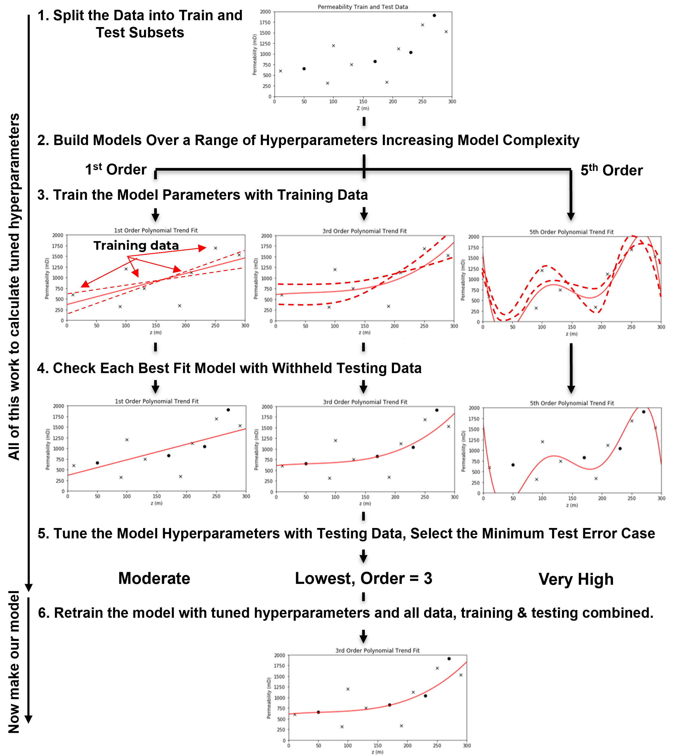
Let’s walk through the key steps,
Train and Test Split - divide the available data into mutually exclusive, exhaustive subsets: a training set and a testing set.
typically, 15%–30% of the data is held out for testing
the remaining 70%–85% is used for training the model
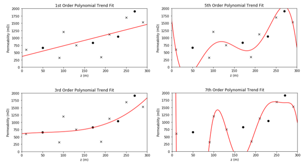
Define a range of hyperparameter(s) values to explore, ranging from,
simple models with low flexibility
to complex models with high flexibility
\(\quad\) This step may involve tuning multiple hyperparameters, in which case efficient sampling methods (e.g., grid search, random search, or Bayesian optimization) are often used.
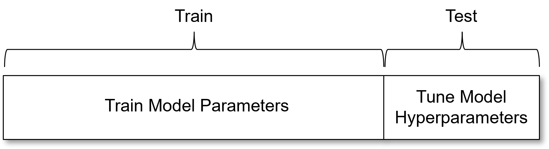
Train Model Parameters for Each Hyperparameter Setting - for each set of hyperparameters, train a model on the training data. This yields:
a suite of trained models, each with different complexity
each model has parameters optimized to minimize error on the training data
Evaluate Each Model on the Withheld Testing Data - using the testing data,
evaluate how each trained model performs on unseen data
summarize prediction error (for example, root mean square error (RMSE), mean absolute error (MAE), classification accuracy) for each model
Select the Hyperparameters That Minimize Test Error - this is the hyperparameter tuning step:
choose the model hyperparaemter(s) that performs best on the test data
these are your tuned hyperparameters
Retrain the Final Model on All Data Using Tuned Hyperparameters - now that the best model complexity has been identified,
retrain the model using both the training and test sets
this maximizes the amount of data used for final model parameter estimation
the resulting model is the one you deploy in real-world applications
Common Questions About the Model Training and Tuning Workflow#
As a professor, I often hear these questions when I introduce the above machine learning model training and tuning workflow.
What is the main outcome of steps 1–5? - the only reliable outcome is the tuned hyperparameters.
\(\quad\) we do not use the model trained in step 3 or 4 directly, because it was trained without access to all available data. Instead, we retrain the final model using all data with the selected hyperparameters.
Why not train the model on all the data from the beginning? - because if we do that, we have no independent way to evaluate the model’s generalization. A very complex model can easily overfit—fitting the training data perfectly, but performing poorly on new, unseen data.
\(\quad\) overfitting happens when model flexibility is too high—it captures noise instead of the underlying pattern. Without a withheld test set, we can’t detect this.
This workflow for training and tuning predictive machine learning models is,
an empirical, cross-validation-based process
a practical simulation of real-world model use
a method to identify the model complexity that best balances fit and generalization
I’ve said model parameters and model hyperparameters a bunch of times, so I owe you their definitions.
Model Parameters and Model Hyperparameters#
Model parameters are fit during training phase to minimize error at the training data, i.e., model parameters are trained with training data and control model fit to the data. For example,
for the polynomial predictive machine learning model from the machine learning workflow example above, the model parameters are the polynomial coefficients, e.g., \(b_3\), \(b_2\), \(b_1\) and \(c\) (often called \(b_0\)) for the third order polynomial model.
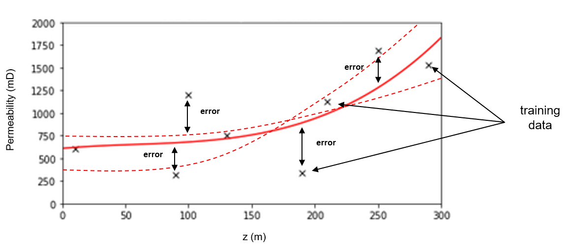
Model hyperparameters are very different. They do not constrain the model fit to the data directly, instead they constrain the model complexity. The model hyperparameters are selected (call tuning) to minimize error at the withheld testing data. Going back to our polynomial predictive machine learning example, the choice of polynomial order is the model hyperparameter.
Model parameters vs. model hyperparameters
Model parameters control the model fit and are trained with training data. Model hyperparameters control the model complexity and are tuned with testing data.
Regression and Classification#
Before we proceed, we need to define regression and classification.
Regression - a predictive machine learning model where the response feature(s) is continuous.
Classification - a predictive machine learning model where the response feature(s) is categorical.
It turns out that for each of these we need to build different models and use different methods to score these models.
for the remainder of this discussion we will focus on regression, but in later chapters we introduce classification models as well.
Now, to better understand predictive machine learning model tuning, i.e., the empirical approach to tune model complexity to minimize testing error, we need to understand the sources of testing error.
the causes of the thing that we are attempting to minimize!
Training and Testing Data#
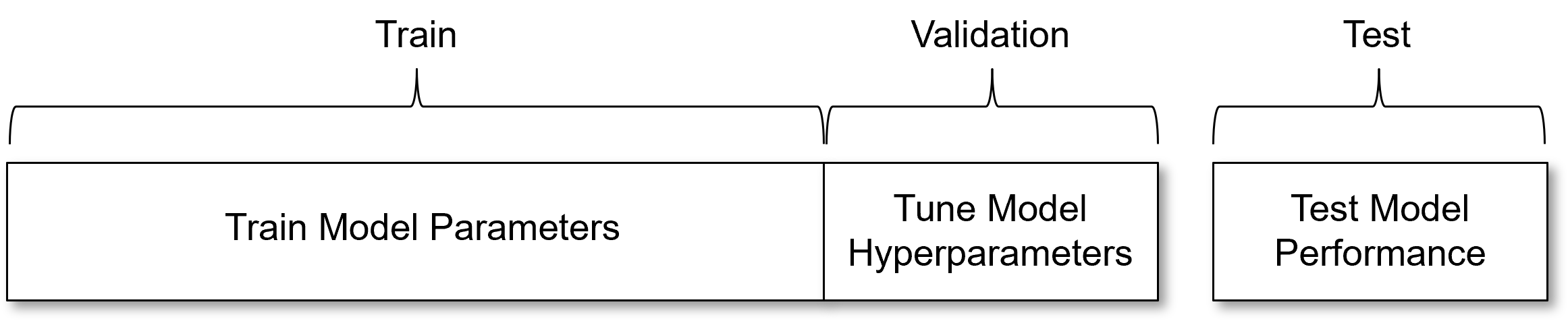
For clarity, consider this is schematic of the flow of training and testing data in the predictive machine learning model parameter training and hyperparameter tuning workflow,

Training Data,
trains model parameters
trains the final model for real world use
Testing Data,
withheld from training model parameters to avoid model overfit
tunes model hyperparameters
returned to train the final tuned model for deployment
How Much Data Should be Withheld for Testing?#
The proportion in testing is recommended by various sources from 15% - 30% of the total dataset. This is a compromise,
data withheld for testing reduces the data available for training; therefore, reduces the accuracy of the model.
data withheld for testing improves the accuracy of the assessment of the model performance.
Various authors have experimented on a variety of training and testing ratios and have recommended splits for their applications,
the optimum ratio of training and testing split depends on problem setting
To determine the proportion of testing data to withheld we could consider the difficulty in model parameter training (e.g., the number of model parameters) and the difficulty in model hyperparameter tuning (e.g., number of hyperparameters, range of response feature outcomes).
Fair Train and Test Splits#
Dr. Julian Salazar suggests that for spatial prediction problems that random train and test data splits may not be fair.
proposed a fair train and test split method for spatial prediction models that splits the data based on the difficulty of the planned use of the model.
prediction difficulty is related to kriging variance that accounts for spatial continuity and distance offset, i.e., the difficulty of the estimate.
the testing split is iterated to match the distribution of kriging variance for planned real world use of the model
To illustrate this concept of prediction difficulty, consider this set of well logs with both random assignment of testing data and withholding an entire contiguous region of the well log for testing data.
easy prediction problem - for random assignment, usually training data are available very close and very similar to the withheld testing data
difficult prediction problem - for removal of the contiguous region, there are no similar nor close training data to the withheld testing data
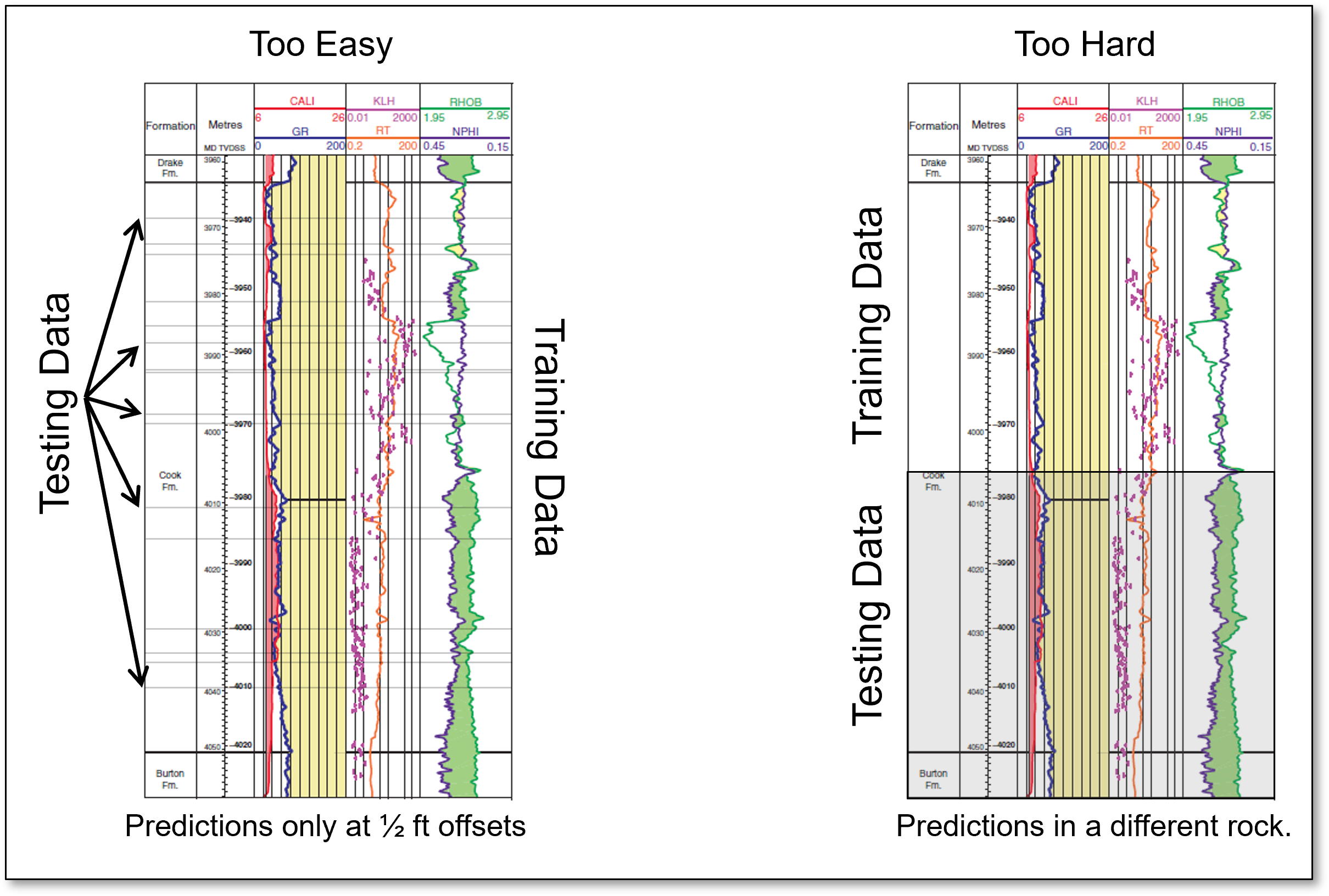
Consider the following prediction cases, i.e., planned real world use of the models, and some practical suggestions for fair train and test split.
If the model will be used to impute data with small offsets from available data then construct a train and test split with train data close to test data - random assignment of withheld testing data is likely sufficient.
if the model will be used to predict a large distance offsets then perform splits the result is large offsets between train and test data - withhold entire wells, drill holes or spatial regions.
Note, with fair train and test splits the tuned model may vary based on the planned use for the model.
Use a simple method like withholding entire wells for a predrill prediction model, or use the Dr. Salazar workflow, but don’t ignore this issue and just use random selection by default.
admittedly, throughout this e-book for demonstration workflow brevity and clarity I have just used random training and testing data assignments.
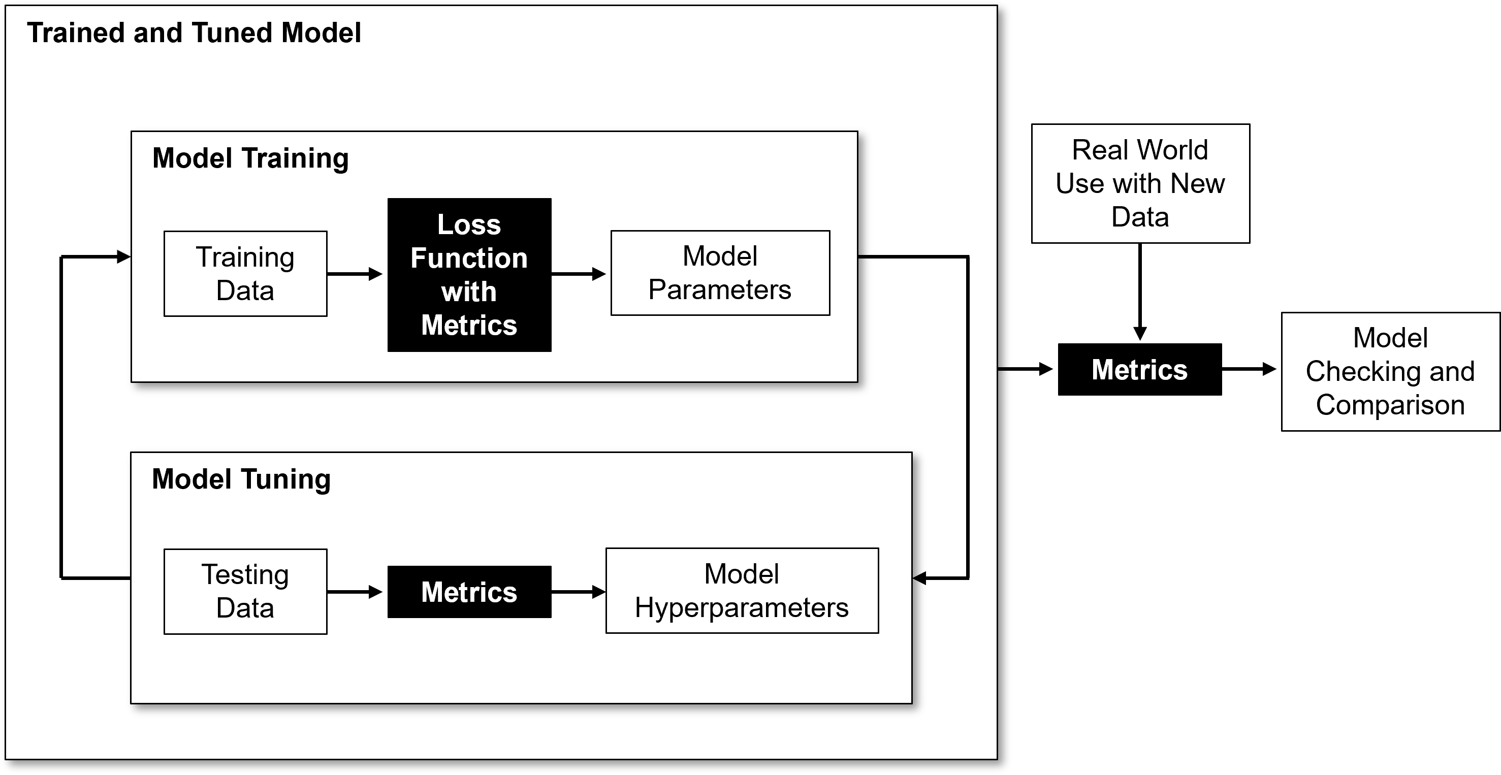
Model Metrics#
Since we have covered the workflows for training and tuning, now we can specify the model metrics that are applied for,
training model parameters
tuning model hyperparameters
model checking and comparison
Here’s an flowchart indicating how these metrics fit into the machine learning modeling workflow.
Choice of model metric depends primarily on the context of the prediction problem,
classification vs. regression
individual estimates vs. entire subsets in space (images) or time (signals)
estimation vs. uncertainty
There are additional considerations, for example,
\(L^1\) vs \(L^2\) norms with their differences, for example, in robustness with outliers, stability of solutions and solution sparsity
consistency with model assumptions, for example, \(r^2\) is only valid for linear models
Let’s review some of the common model metrics for regression models and then for classification models.
Mean Square Error (MSE)#
Is sensitive to outliers, but is continuously differentiable, leading to a closed-form expression for model training. Since the error is squared the error units are squared and this may be less interpretable, for example, MSE of 23,543 \(mD^2\). The equation is,
Mean Absolute Error (MAE)#
Is robust in the presence of outliers, but is not continuously differentiable; therefore, there is no closed-form expression for model training and training is generally accomplished by iterative optimization. The equation is,
Variance Explained#
The proportion of variance of the response feature captured by the model. Assumes additivity of variance; therefore, we only use this model metric for linear models.
First we calculate the variance explained by the model, simply as the variance of the model predictions,
then we calculate the variance not explained by the model as the variance of the error over the model predictions,
then under the assumption of additivity of variance, we calculate the ratio of variance explained over all variance, variance explained plus variance not explained,
For linear regression, recall \(r^2 = \left( \rho_(X,y) \right)^2\); therefore, like correlation coefficients, \(r^2\),
has similar issues as correlation with respect to outliers and mixing multiple populations, e.g., Simpson’s Paradox
for nonlinear models consider pseudo-R-square methods
Also, even a linear model can have a negative \(r^2\) if the model trend contradicts the data trend, for example, if you fit data with a negative slope with a linear model with a positive slope!
Inlier Ratio#
The proportion of testing data, \(y_i\) within a margin, \(\epsilon\), of the model, \(\hat{y}_i\), calculated as,
where the indicator transform, \(I_R\) is defined as,
Here’s an illustration of the inlier ratio model metric, \(I_R\) model metric,
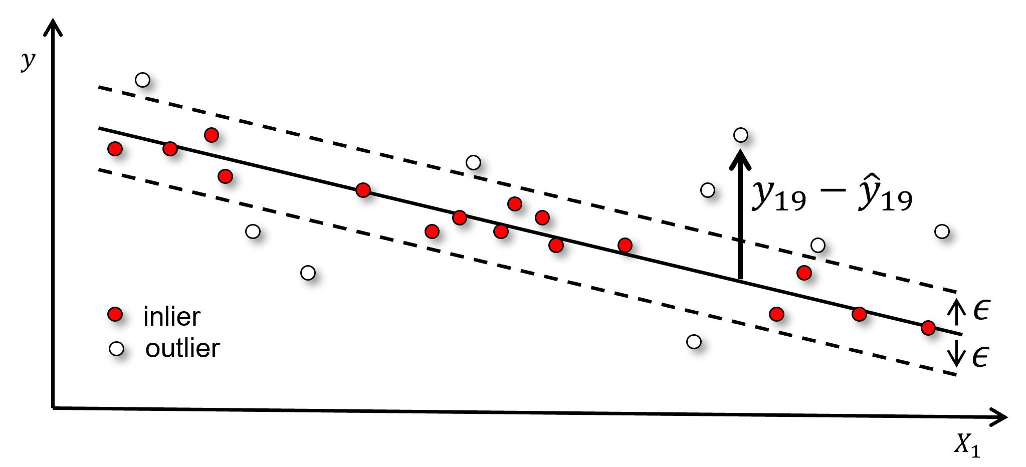
While the illustration is a linear model, this metric may be applied to any model. Although there is some subjectivity with the inlier ratio model metric,
what is the best selection for the margin, \(\epsilon\)?
Common Classification Model Metrics#
Let’s review some of the common model metrics for classification models. Classification is potentially more complicated than regression, since instead of a single model metric, we actually calculate an entire confusion matrix,
a \(K \times K\) matrix with frequencies of predicted (x axis) vs. actual (y axis) categories to visualize the performance of a classification model, where \(K\) is the response feature cardinality, i.e., the number of possible categories
visualize and diagnose all the combinations of correct and misclassification with the classification model, for example, category 1 is often misclassified as category 3,
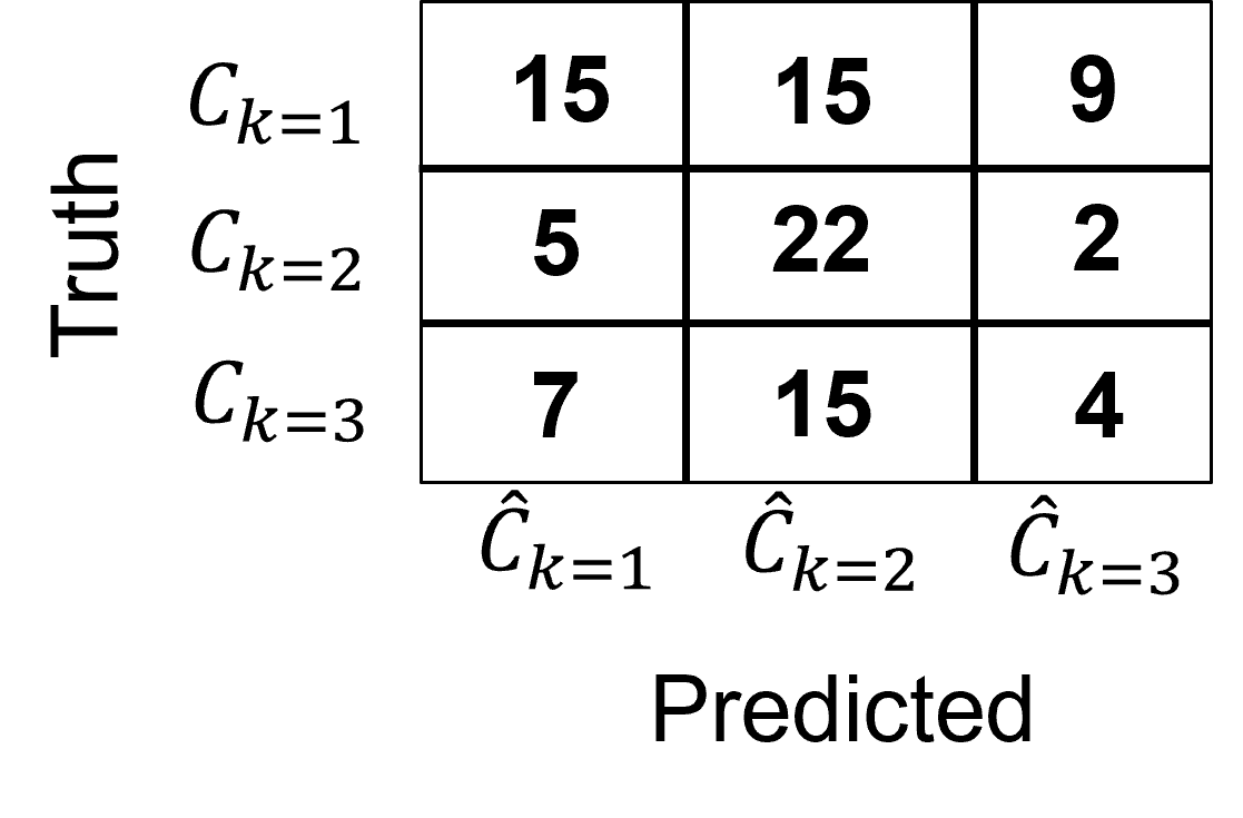
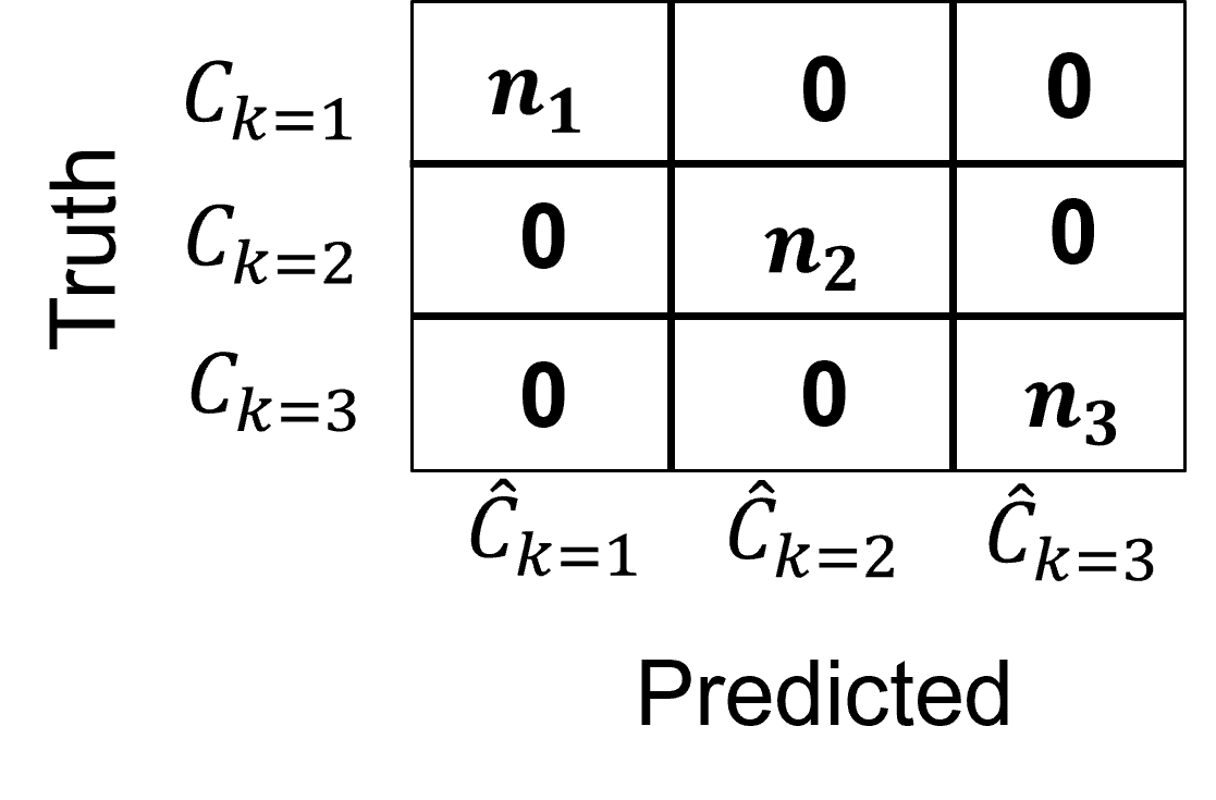
perfect accuracy is number of each class, \(n_1, n_2, \ldots, n_K\) on the diagonal, i.e., category 1 is always predicted as category 1, etc.
the confusion matrix is applied to calculate a single summary of categorical accuracy, for example, precision, recall, etc.
model metrics are specific to the specific category and may significantly vary over categories, i.e., we can predict well for category \(k=1\) but not for category \(k=3\).
Precision#
For category \(𝑘\), precision is the ratio of true positive over all positives,
we can intuitively describe precision as the conditional probability,
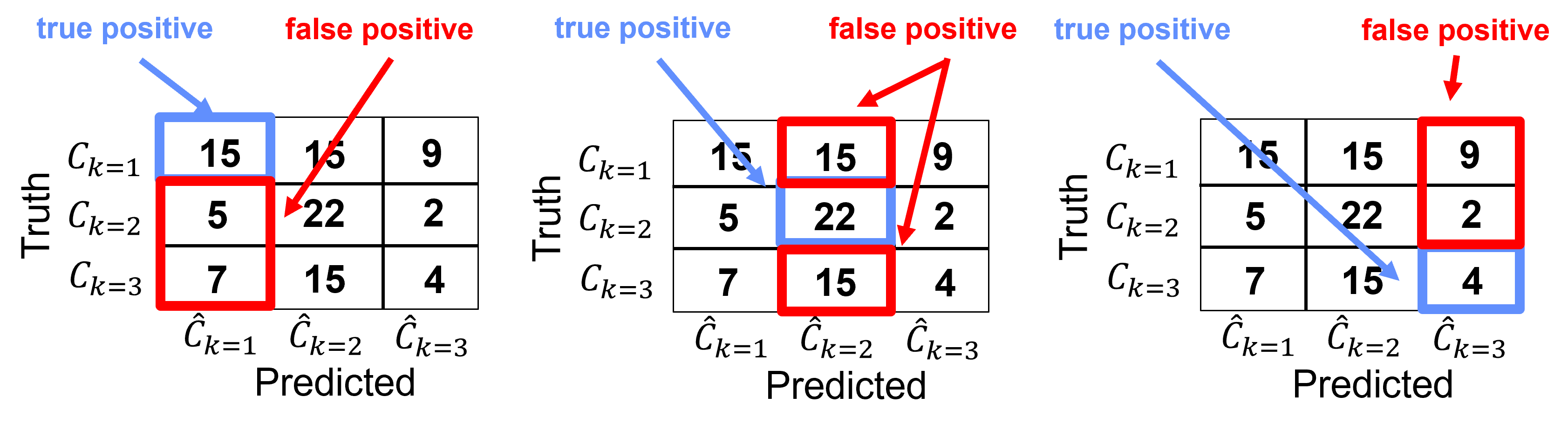
For this example, we can calculate the precision for each category as,
Category k=1
Category k = 2,
Category k = 3,
Recall (called sensitivity in medical)#
Recall for group \(𝑘\) is the ratio of true positives over all cases of \(𝑘\).
We can intuitively describe recall as, how many of group 𝑘 did we catch?
Note, recall does not account for false positives.
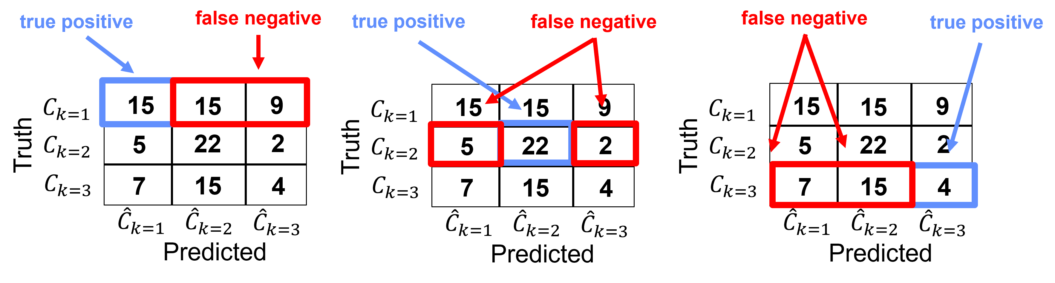
For this example, we can calculate the recall for each category as,
Category k=1
Category k = 2,
Category k = 3,
Specificity#
Specificity for group \(𝑘\) is the ratio of true negatives over all negative cases of \(n \ne 𝑘\).
We can intuitively describe specificity as, how many of not group \(k\) did we catch?
Note, recall does not account for true positives.
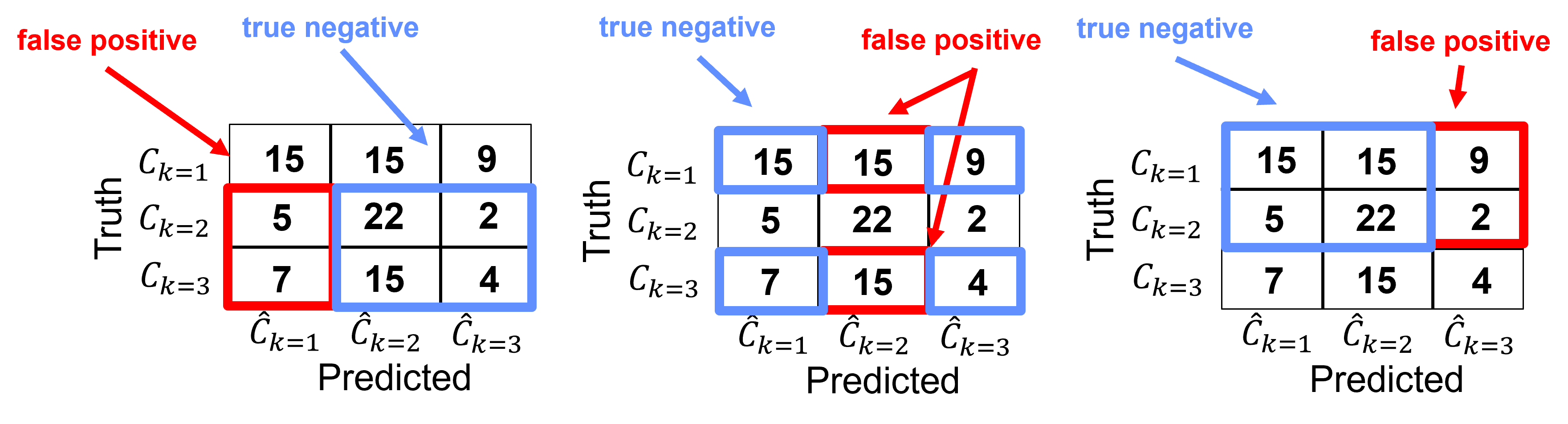
For this example, we can calculate the recall for each category as,
Category k=1
Category k = 2,
Category k = 3,
f1-score#
f1-score is the harmonic mean of precision and recall for each \(k\) category,
The idea is to combine precision and recall into a single metric since they both see different aspects of the classification model accuracy.
the harmonic mean is sensitive the to lowest score; therefore, good performance in one score cannot average out or make up for bad performance in the other
Train and Test Hold Out Cross Validation#
If only one train and test data split is applied to tune our machine learning model hyperparameters then we are applying the hold out cross validation approach.
we split the data into training and testing data, these are exhaustive and mutually exclusive groups.
but this cross validation method is not exahustive, we only consider the one split for testing, most data are not tested. Also, we do not explore the full combinatorial of possible splits (more about this as we compare with other cross validation methods)
The workflow is,
withhold the testing data subset from model training
train models with the remaining training data with various hyperparameters representing simple to complicated models
then test the suite of simple to complicated trained models with withheld testing data
select the model hyperparameters (complexity) with lowest testing error
retrain the model with the turned hyperparameters and all of the data for deployment
The advantage of this approach is that we can readily evaluate the training and testing data split.
since there is only one split, we can easily visualize and evaluate the train and test data cases, coverage and balance
The disadvantage is that this method may be sensitive to the specific selection of testing data
as a result hold out cross validation may result in a noisy plot of testing error vs. the hyperparameter
Train, Validate and Test Hold Out Cross Validation#
There is a more complete hold out cross validation workflow commonly applied,
Train with training data split - models sees and learns from this data to train the model parameters.
Validate with the validation data split - evaluation of model complexity vs. accuracy with data withheld from model parameter training to tune the model hyperparameters. The same as testing data in train and test workflow.
Test model performance with testing data - data withheld until the model is complete to provide a final evaluation of model performance. This data had no role in building the model and is commonly applied to compare multiple competing models.
I understand the motivation for the training, validation and testing cross validation workflow. It is an attempt to check our models, objectively, with cases that,
we know the truth and can access accuracy accurately
had nothing to do with the model construction, training model parameters nor tuning model hyperparameters
I appreciate this, but I have some concerns,
We are further reducing the number of samples available to training model parameters and to tuning model hyperparameters.
Eventually we will retrain the tuned model with all the data, so the model we test is not actually the final deployed model.
What do we do if the testing data is not accurately predicted? Do we include another round of testing with another withheld subset of the data? Ad infinitum?
Load the Required Libraries#
The following code loads the required libraries. These should have been installed with Anaconda 3.
ignore_warnings = True
import pandas as pd
import numpy as np
import matplotlib.pyplot as plt
from matplotlib.ticker import (MultipleLocator, AutoMinorLocator) # control of axes ticks
from sklearn.model_selection import cross_val_score           # multi-processor K-fold crossvalidation
from sklearn.model_selection import train_test_split          # train and test split
from sklearn.model_selection import KFold                     # K-fold cross validation
plt.rc('axes', axisbelow=True)                                # plot all grids below the plot elements
if ignore_warnings == True:
    import warnings
    warnings.filterwarnings('ignore')
cmap = plt.cm.inferno                                         # color map
seed = 42                                                     # random number seed
Declare Functions#
I also added a convenience function to add major and minor gridlines to improve plot interpretability.
def add_grid():
    plt.gca().grid(True, which='major',linewidth = 1.0); plt.gca().grid(True, which='minor',linewidth = 0.2) # add y grids
    plt.gca().tick_params(which='major',length=7); plt.gca().tick_params(which='minor', length=4)
    plt.gca().xaxis.set_minor_locator(AutoMinorLocator()); plt.gca().yaxis.set_minor_locator(AutoMinorLocator()) # turn on minor ticks
Load Data to Demonstration Cross Validation Methods#
Let’s load a spatial dataset and select 2 predictor features to visualize cross validation methods.
we will focus on the data splits and not the actual model training and tuning. Later when we cover predictive machine learning methods we will add the model component of the workflow.
df = pd.read_csv('https://raw.githubusercontent.com/GeostatsGuy/GeoDataSets/master/unconv_MV_v4.csv') # load data from Dr. Pyrcz's GitHub repository

response = 'Prod'                                             # specify the response feature
X = df.iloc[:,[1,3]]                                          # make predictor and response DataFrames
y = df.loc[:,response]

Xname = X.columns.values.tolist()                             # store the names of the features
yname = y.name

Xmin = [6.0,1.0]; Xmax = [24.0,5.0]                           # set the minimum and maximum values for plotting
ymin = 500.0; ymax = 9000.0

Xlabel = ['Porosity','Acoustic Impedance']
ylabel = 'Normalized Initial Production (MCFPD)'

Xtitle = ['Porosity','Acoustic Impedance']
ytitle = 'Normalized Initial Production'

Xunit = ['%',r'$kg/m^3 x m/s x 10^3$']; yunit = 'MCFPD'
Xlabelunit = [Xlabel[0] + ' (' + Xunit[0] + ')',Xlabel[1] + ' (' + Xunit[1] + ')']
ylabelunit = ylabel + ' (' + yunit + ')'

m = len(pred) + 1
mpred = len(pred)
---------------------------------------------------------------------------
NameError                                 Traceback (most recent call last)
Cell In[3], line 23
     20 Xlabelunit = [Xlabel[0] + ' (' + Xunit[0] + ')',Xlabel[1] + ' (' + Xunit[1] + ')']
     21 ylabelunit = ylabel + ' (' + yunit + ')'
---> 23 m = len(pred) + 1
     24 mpred = len(pred)

NameError: name 'pred' is not defined
Visualize Train and Test Hold Out Cross Validation#
Let’s compare the train and test with train, validate and test hold out data splits.
first we plot a train and test data split and then a train, validate and test split.
test_prop = 0.15                                              # set the proportion of test data to withhold
X_train, X_test, y_train, y_test = train_test_split(X,y,test_size=test_prop,random_state=73073) # train and test split
df_train = pd.concat([X_train,y_train],axis=1)                # make one train DataFrame with both X and y (remove all other features)
df_test = pd.concat([X_test,y_test],axis=1)                   # make one testin DataFrame with both X and y (remove all other features)

nbins = 20                                                    # number of histogram bins

plt.subplot(221)                                              # predictor feature #1 histogram
freq1,_,_ = plt.hist(x=df_train[Xname[0]],weights=None,bins=np.linspace(Xmin[0],Xmax[0],nbins),alpha = 0.6,
                     edgecolor='black',color='darkorange',density=False,label='Train')
freq2,_,_ = plt.hist(x=df_test[Xname[0]],weights=None,bins=np.linspace(Xmin[0],Xmax[0],nbins),alpha = 0.6,
                     edgecolor='black',color='red',density=False,label='Test')
max_freq = max(freq1.max()*1.10,freq2.max()*1.10)
plt.xlabel(Xlabelunit[0]); plt.ylabel('Frequency'); plt.ylim([0.0,max_freq]); plt.title(Xtitle[0]); add_grid()
plt.xlim([Xmin[0],Xmax[0]]); plt.legend(loc='upper right')

plt.subplot(222)                                              # predictor feature #2 histogram
freq1,_,_ = plt.hist(x=df_train[Xname[1]],weights=None,bins=np.linspace(Xmin[1],Xmax[1],nbins),alpha = 0.6,
                     edgecolor='black',color='darkorange',density=False,label='Train')
freq2,_,_ = plt.hist(x=df_test[Xname[1]],weights=None,bins=np.linspace(Xmin[1],Xmax[1],nbins),alpha = 0.6,
                     edgecolor='black',color='red',density=False,label='Test')
max_freq = max(freq1.max()*1.10,freq2.max()*1.10)
plt.xlabel(Xlabelunit[1]); plt.ylabel('Frequency'); plt.ylim([0.0,max_freq]); plt.title(Xtitle[1]); add_grid()
plt.xlim([Xmin[1],Xmax[1]]); plt.legend(loc='upper right')

plt.subplot(223)                                              # predictor feature #2 histogram
freq1,_,_ = plt.hist(x=df_train[yname],weights=None,bins=np.linspace(ymin,ymax,nbins),alpha = 0.6,
                     edgecolor='black',color='darkorange',density=False,label='Train')
freq2,_,_ = plt.hist(x=df_test[yname],weights=None,bins=np.linspace(ymin,ymax,nbins),alpha = 0.6,
                     edgecolor='black',color='red',density=False,label='Test')
max_freq = max(freq1.max()*1.10,freq2.max()*1.10)
plt.xlabel(ylabelunit); plt.ylabel('Frequency'); plt.ylim([0.0,max_freq]); plt.title(ytitle); add_grid()
plt.xlim([ymin,ymax]); plt.legend(loc='upper right')

plt.subplot(224)                                              # predictor features #1 and #2 scatter plot
plt.scatter(df_train[Xname[0]],df_train[Xname[1]],s=40,marker='o',color = 'darkorange',alpha = 0.8,edgecolor = 'black',zorder=10,label='Train')
plt.scatter(df_test[Xname[0]],df_test[Xname[1]],s=40,marker='o',color = 'red',alpha = 0.8,edgecolor = 'black',zorder=10,label='Test')
plt.title(Xlabel[0] + ' vs ' +  Xlabel[1])
plt.xlabel(Xlabelunit[0]); plt.ylabel(Xlabelunit[1])
plt.legend(); add_grid(); plt.xlim([Xmin[0],Xmax[0]]); plt.ylim([Xmin[1],Xmax[1]])

plt.subplots_adjust(left=0.0, bottom=0.0, right=2.0, top=2.1, wspace=0.3, hspace=0.2)
#plt.savefig('Test.pdf', dpi=600, bbox_inches = 'tight',format='pdf')
plt.show()
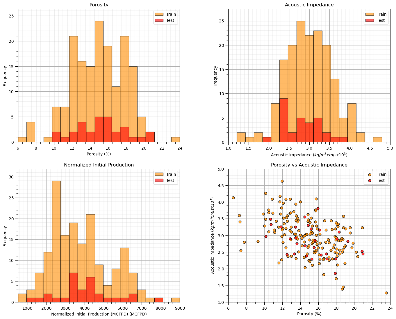
It is a good idea to visualize the train and test split,
histograms for each predictor feature and the response feature to ensure that the train and test cover the range of possible outcomes and are balanced
if the number of predictor features is 2 then we can actually plot the predictor feature space to check coverage and balance of train and test data splits
Now let’s repeat this for the train, validate and test data split.
val_prop = 0.15; test_prop = 0.15                             # set the proportion of test data to withhold
nbins = 20                                                    # number of histogram bins

X_train, X_temp, y_train, y_temp = train_test_split(X, y, test_size=val_prop + test_prop, random_state=42)
X_val, X_test, y_val, y_test = train_test_split(X_temp, y_temp, test_size=test_prop/(val_prop + test_prop), random_state=42)

df_train = pd.concat([X_train,y_train],axis=1); df_val = pd.concat([X_val,y_val],axis=1); df_test = pd.concat([X_test,y_test],axis=1)

plt.subplot(221)                                              # predictor feature #1 histogram
freq1,_,_ = plt.hist(x=df_train[Xname[0]],weights=None,bins=np.linspace(Xmin[0],Xmax[0],nbins),alpha = 0.6,
                     edgecolor='black',color='darkorange',density=False,label='Train')
freq2,_,_ = plt.hist(x=df_val[Xname[0]],weights=None,bins=np.linspace(Xmin[0],Xmax[0],nbins),alpha = 0.6,
                     edgecolor='black',color='red',density=False,label='Validate')
freq3,_,_ = plt.hist(x=df_test[Xname[0]],weights=None,bins=np.linspace(Xmin[0],Xmax[0],nbins),alpha = 0.6,
                     edgecolor='black',color='blue',density=False,label='Test')
max_freq = max(freq1.max()*1.10,freq2.max()*1.10,freq3.max()*1.10)
plt.xlabel(Xlabelunit[0]); plt.ylabel('Frequency'); plt.ylim([0.0,max_freq]); plt.title(Xtitle[0]); add_grid()
plt.xlim([Xmin[0],Xmax[0]]); plt.legend(loc='upper right')

plt.subplot(222)                                              # predictor feature #2 histogram
freq1,_,_ = plt.hist(x=df_train[Xname[1]],weights=None,bins=np.linspace(Xmin[1],Xmax[1],nbins),alpha = 0.6,
                     edgecolor='black',color='darkorange',density=False,label='Train')
freq2,_,_ = plt.hist(x=df_val[Xname[1]],weights=None,bins=np.linspace(Xmin[1],Xmax[1],nbins),alpha = 0.6,
                     edgecolor='black',color='red',density=False,label='Validate')
freq3,_,_ = plt.hist(x=df_test[Xname[1]],weights=None,bins=np.linspace(Xmin[1],Xmax[1],nbins),alpha = 0.6,
                     edgecolor='black',color='blue',density=False,label='Test')
max_freq = max(freq1.max()*1.10,freq2.max()*1.10,freq3.max()*1.10)
plt.xlabel(Xlabelunit[1]); plt.ylabel('Frequency'); plt.ylim([0.0,max_freq]); plt.title(Xtitle[1]); add_grid()
plt.xlim([Xmin[1],Xmax[1]]); plt.legend(loc='upper right')

plt.subplot(223)                                              # predictor feature #2 histogram
freq1,_,_ = plt.hist(x=df_train[yname],weights=None,bins=np.linspace(ymin,ymax,nbins),alpha = 0.6,
                     edgecolor='black',color='darkorange',density=False,label='Train')
freq2,_,_ = plt.hist(x=df_val[yname],weights=None,bins=np.linspace(ymin,ymax,nbins),alpha = 0.6,
                     edgecolor='black',color='red',density=False,label='Validate')
freq2,_,_ = plt.hist(x=df_test[yname],weights=None,bins=np.linspace(ymin,ymax,nbins),alpha = 0.6,
                     edgecolor='black',color='blue',density=False,label='Test')
max_freq = max(freq1.max()*1.10,freq2.max()*1.10,freq3.max()*1.10)
plt.xlabel(ylabelunit); plt.ylabel('Frequency'); plt.ylim([0.0,max_freq]); plt.title(ytitle); add_grid()
plt.xlim([ymin,ymax]); plt.legend(loc='upper right')

plt.subplot(224)                                              # predictor features #1 and #2 scatter plot
plt.scatter(df_train[Xname[0]],df_train[Xname[1]],s=40,marker='o',color = 'darkorange',alpha = 0.8,edgecolor = 'black',zorder=10,label='Train')
plt.scatter(df_val[Xname[0]],df_val[Xname[1]],s=40,marker='o',color = 'blue',alpha = 0.8,edgecolor = 'black',zorder=10,label='Test')
plt.scatter(df_test[Xname[0]],df_test[Xname[1]],s=40,marker='o',color = 'red',alpha = 0.8,edgecolor = 'black',zorder=10,label='Test')
plt.title(Xlabel[0] + ' vs ' +  Xlabel[1])
plt.xlabel(Xlabelunit[0]); plt.ylabel(Xlabelunit[1])
plt.legend(); add_grid(); plt.xlim([Xmin[0],Xmax[0]]); plt.ylim([Xmin[1],Xmax[1]])

plt.subplots_adjust(left=0.0, bottom=0.0, right=2.0, top=2.1, wspace=0.3, hspace=0.2)
#plt.savefig('Test.pdf', dpi=600, bbox_inches = 'tight',format='pdf')
plt.show()
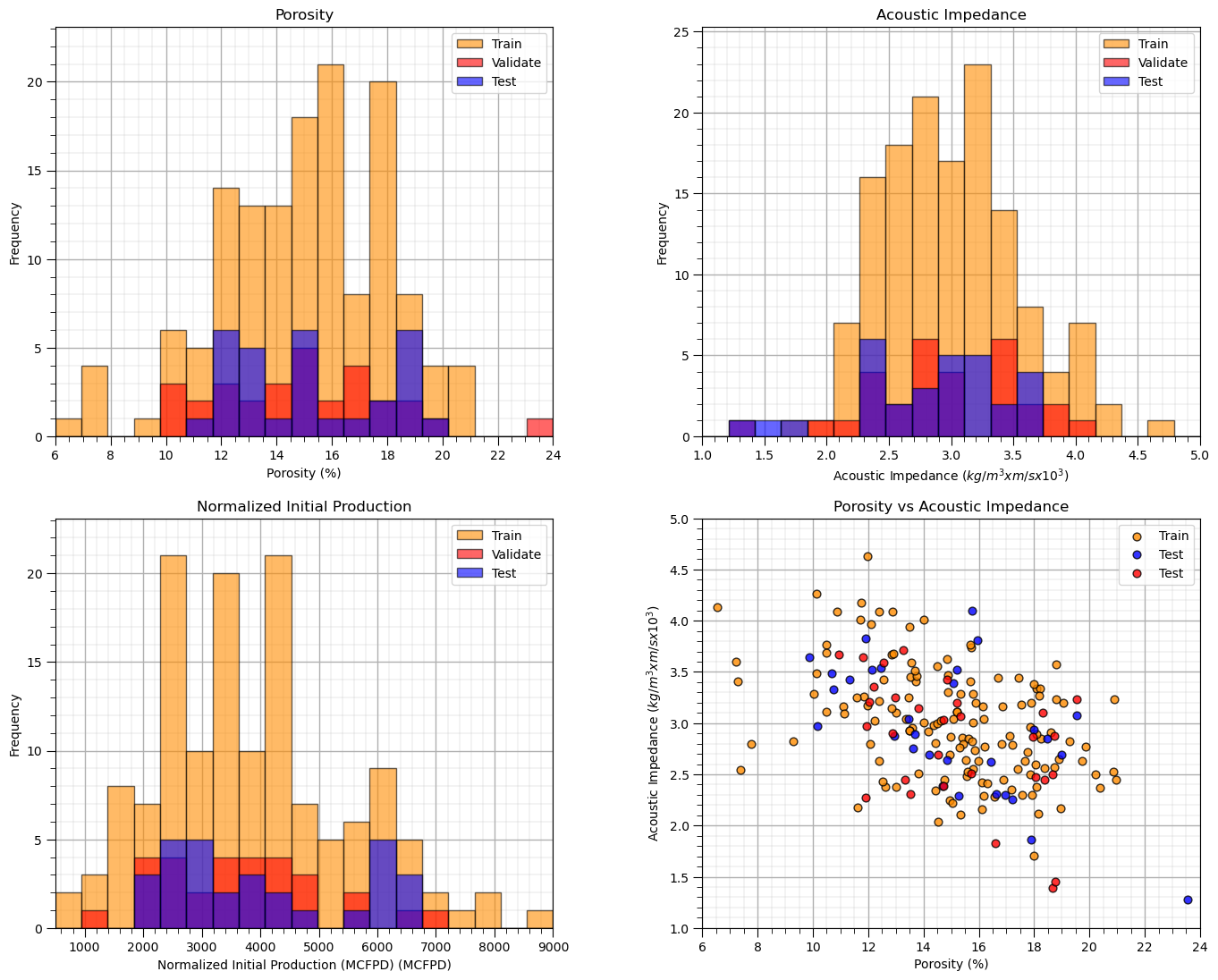
Once again we can visualize the splits, now train, validate and test,
histograms for each predictor feature and the response feature to ensure that the train and test cover the range of possible outcomes and are balanced
if the number of predictor features is 2 then we can actually plot the predictor feature space to check coverage and balance of train and test data splits
Leave-one-out Cross Validation (LOO CV)#
Leave-one-out cross validation is an exhaustive cross validation method, i.e., all data gets tested by loop over all the data.
we train and tune \(n\) models, for each model a single datum is withheld as testing and the \(n-1\) data are assigned as training data
we will calculate \(n\) training and testing errors that will be aggregated over all \(n\) models, for example, the average of the mean square error.
In the case of leave-one-out cross validation,
we test at only one datum so the test error is just a single error at the single withheld datum, so we just use standard MSE over the \(n\) models
but, we have \(n-1\) training data for each model, so we aggregate, by averageing the mean square error of each model,
Here’s the leave-one-out cross validation steps,
Loop over all \(n\) data, and withhold that data
Train on the remaining \(n−1\) data and test on the withheld single data
Calculate model goodness metric, MSE for a single test data is the square error
Goto 1
Aggregate model goodness metric over all data, \(n\)
Typically, leave-one-out cross validation is too easy of a prediction problem; therefore, it is not commonly used,
but it introduces the concept of exhaustive cross validation, i.e., all data gets tested!
Leave-one-out cross validation is also exhaustive in the sense that the full combinatorial of \(n\) data choose \(p\) where \(p=1\) are explored,
where the full combinatorial is the \(n\) models that we built above!
K-fold Cross Validation (k-fold CV)#
K-fold is a more general, efficient and robust approach.
a exhaustive cross validation approach (all data are tested), but it samples a limited set of the possible combinatorial of prediction problems, unlike Leave-one-out cross validation where we attempt every possible case on data withheld for testing
for K-fold cross validation we assign a single set of K equal size splits and we loop over the splits, withholding the \(k\) split for testing data and using the data outside the split for training
the testing proportion is \(\frac{1}{K}\), e.g., for \(K=3\), 33.3% is withheld for testing, for \(K=4\), 25% is withheld for testing and for \(K=5\), 20% is withheld for testing
We call it K-fold cross validation, because each of the splits is known as a fold. Here’s the steps for K-fold cross validation,
Select \(K\), integer number of folds
Split the data into \(K\) equal size folds
Loop over each \(k = 1,\ldots,K\) fold
Assign the data outside the \(k\) fold as training data and inside the \(k\) fold as testing data
Train and test the prediction model and calculated the testing model metric
Goto 3
Aggregate testing model metric over all K folds
As you can see above k-fold cross validation is exhaustive, since all data is tested, i.e., withheld as testing data, but the method is not exhaustive in that all possible \(\frac{n}{K}\) data subsets are not considered.
To calculated the combinatorial for exhaustive K folds we used the multinomial coefficient,
For example, if there are \(n=100\) data and \(K=4\) folds, there are \(6.72 \times 10^55\) possible combinations. I vote that we stick with regular K-fold cross validation.
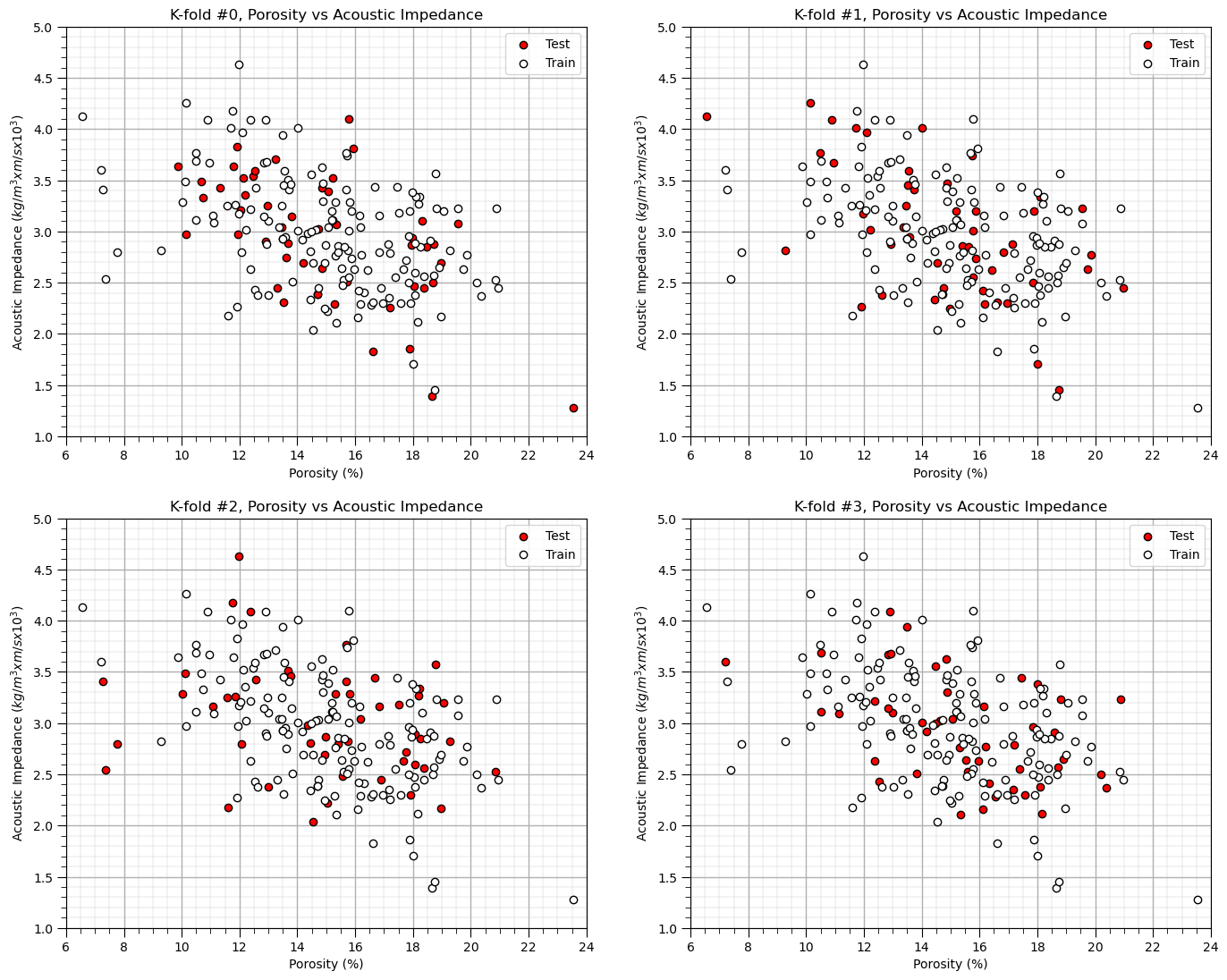
Let’s visualize K-fold cross validation splits, for the case of \(K=4\).
K = 4
kf = KFold(n_splits=K, shuffle=True, random_state=seed)

df['Fold'] = -1
for fold_number, (train_index, test_index) in enumerate(kf.split(df)):
    df.loc[test_index, 'Fold'] = fold_number  # Assign fold number to test set

for k in range(0,K):
    df_in = df[df['Fold'] == k]; df_out = df[df['Fold'] != k]
    plt.subplot(2,2,k+1)
    plt.scatter(df_in[Xname[0]],df_in[Xname[1]],color='red',edgecolor='black',label='Test')
    plt.scatter(df_out[Xname[0]],df_out[Xname[1]],color='white',edgecolor='black',label='Train'); add_grid()
    plt.title('K-fold #' + str(k) + ', ' + Xlabel[0] + ' vs ' +  Xlabel[1])
    plt.xlabel(Xlabelunit[0]); plt.ylabel(Xlabelunit[1])
    plt.legend(); add_grid(); plt.xlim([Xmin[0],Xmax[0]]); plt.ylim([Xmin[1],Xmax[1]])

plt.subplots_adjust(left=0.0, bottom=0.0, right=2.0, top=2.1, wspace=0.2, hspace=0.2); plt.show()
Leave-p-out Cross Validation (LpO-CV)#
This is the variant of K-fold cross validation that exhaustively samples the full combinatorial of withholding \(p\) testing data.
Select \(p\), integer number of testing data to withhold
For all possible \(p\) subsets of \(n\),
Assign the data outside the \(p\) as training data and inside the \(p\) as testing data
Train and test the prediction model and calculated the testing model metric
Goto 2
Aggregate testing model metric over the combinatorial
For this case the combinatorial of cases is, \(n\) choose \(p\),
For \(n=100\) and \(p=20\), we have \(5.36 \times 10^{20}\) combinations to check!
Limitations of Cross Validation#
Here are some additional issues with the model cross validation approach in general,
Peeking, Information Leakage – some information is transmitted from the withheld data into the model, some model decision(s) use all the data. Pipelines and wrappers help with this.
Black Swans / Stationarity – the model cannot be tested for data events not available in the data. This is also known as the ‘No Free Lunch Theorem’ in machine learning
Consider the words of Hume,
“even after the observation of the frequent or constant conjunction of objects, we have no reason to draw any inference concerning any object beyond those of which we have had experience” - Hume (1739–1740)
We cannot predict things that we have never seen in our data!
here’s a quote from the famous Oreskes et al. (1994) paper on subsurface validation and verification,
“Verification and validation of numerical models of natural systems is impossible. This is because natural systems are never closed and because model results are always nonunique. Models can be confirmed by the demonstration of agreement between observation and prediction, but confirmation is inherently partial. Complete confirmation is logically precluded by the fallacy of affirming the consequent and by incomplete access to natural phenomena. Models can only be evaluated in relative terms, and their predictive value is always open to question. The primary value of models is heuristic.”
Oreskes et al. (1994)
all of this is summed up very well with,
‘All models are wrong, but some are useful’ – George Box
and a reminder of,
Parsimony – since all models are wrong, an economical description of the system. Occam’s Razor
resulting in a pragmatic approach of,
Worrying Selectively – since all models are wrong, figure out what is most importantly wrong.
finally, I add my own words,
‘Be humble, the earth will surprise you!’ – Michael Pyrcz
About the Author#

Michael Pyrcz is a professor in the Cockrell School of Engineering, and the Jackson School of Geosciences, at The University of Texas at Austin, where he researches and teaches subsurface, spatial data analytics, geostatistics, and machine learning. Michael is also,
the principal investigator of the Energy Analytics freshmen research initiative and a core faculty in the Machine Learn Laboratory in the College of Natural Sciences, The University of Texas at Austin
an associate editor for Computers and Geosciences, and a board member for Mathematical Geosciences, the International Association for Mathematical Geosciences.
Michael has written over 70 peer-reviewed publications, a Python package for spatial data analytics, co-authored a textbook on spatial data analytics, Geostatistical Reservoir Modeling and author of two recently released e-books, Applied Geostatistics in Python: a Hands-on Guide with GeostatsPy and Applied Machine Learning in Python: a Hands-on Guide with Code.
All of Michael’s university lectures are available on his YouTube Channel with links to 100s of Python interactive dashboards and well-documented workflows in over 40 repositories on his GitHub account, to support any interested students and working professionals with evergreen content. To find out more about Michael’s work and shared educational resources visit his Website.
Want to Work Together?#
I hope this content is helpful to those that want to learn more about subsurface modeling, data analytics and machine learning. Students and working professionals are welcome to participate.
Want to invite me to visit your company for training, mentoring, project review, workflow design and / or consulting? I’d be happy to drop by and work with you!
Interested in partnering, supporting my graduate student research or my Subsurface Data Analytics and Machine Learning consortium (co-PIs including Profs. Foster, Torres-Verdin and van Oort)? My research combines data analytics, stochastic modeling and machine learning theory with practice to develop novel methods and workflows to add value. We are solving challenging subsurface problems!
I can be reached at mpyrcz@austin.utexas.edu.
I’m always happy to discuss,
Michael
Michael Pyrcz, Ph.D., P.Eng. Professor, Cockrell School of Engineering and The Jackson School of Geosciences, The University of Texas at Austin
More Resources Available at: Twitter | GitHub | Website | GoogleScholar | Geostatistics Book | YouTube | Applied Geostats in Python e-book | Applied Machine Learning in Python e-book | LinkedIn
Comments#
This was a basic description of machine learning concepts. Much more could be done and discussed, I have many more resources. Check out my shared resource inventory and the YouTube lecture links at the start of this chapter with resource links in the videos’ descriptions.
I hope this was helpful,
Michael