

Generative Adversarial Networks#
Michael J. Pyrcz, Professor, The University of Texas at Austin
Twitter | GitHub | Website | GoogleScholar | Geostatistics Book | YouTube | Applied Geostats in Python e-book | Applied Machine Learning in Python e-book | LinkedIn
Chapter of e-book “Applied Machine Learning in Python: a Hands-on Guide with Code”.
Cite this e-Book as:
Pyrcz, M.J., 2024, Applied Machine Learning in Python: A Hands-on Guide with Code [e-book]. Zenodo. doi:10.5281/zenodo.15169138 ![]()
The workflows in this book and more are available here:
Cite the MachineLearningDemos GitHub Repository as:
Pyrcz, M.J., 2024, MachineLearningDemos: Python Machine Learning Demonstration Workflows Repository (0.0.3) [Software]. Zenodo. DOI: 10.5281/zenodo.13835312. GitHub repository: GeostatsGuy/MachineLearningDemos ![]()
By Michael J. Pyrcz
© Copyright 2024.
This chapter is a tutorial for / demonstration of Generative Adversarial Networks.
YouTube Lecture: check out my lectures on:
Generative Adversarial Networks (TBA)
These lectures are all part of my Machine Learning Course on YouTube with linked well-documented Python workflows and interactive dashboards. My goal is to share accessible, actionable, and repeatable educational content. If you want to know about my motivation, check out Michael’s Story.
Motivation#
What if we put together machines? Working in a competitive, adversarial manner?
Could we make a more powerful machine learning model that learns its own loss function!
Could we make images that don’t collapse to exact reproduction of the images in the training set?
Generative neural networks are very powerful, nature inspired computing deep learning method to make fake, but realistic, images by application of convolutional neural networks, an analogy of visual cortex that extend the ability of our artificial neural networks to better work with images.
Nature inspired computing is looking to nature for inspiration to develop novel problem-solving methods,
artificial neural networks are inspired by biological neural networks
nodes in our model are artificial neurons, simple processors
connections between nodes are artificial synapses
perceptive fields regularization to improve generalization and efficiency
intelligence emerges from many connected simple processors. For the remainder of this chapter, I will used the terms nodes and connections to describe our convolutional neural network.
Artificial and Convolutional Neural Networks#
If you have not, take this opportunity to review my previous chapters in the e-book on,
The main takeaways from my artificial neural network chapter are as follows,
architecture of a neural network, including its fundamental components, nodes (neurons) and the weighted connections between them.
forward pass computation through the network, where each node computes a weighted sum of its inputs (including a bias term), followed by the application of a nonlinear activation function.
computation of the error derivative, which is then backpropagated through the network via the chain rule to determine the gradients of the loss function with respect to each weight and bias.
aggregation of these gradients across all samples in a training batch, typically by averaging, to update the model parameters.
iterative training process, where the model is trained over multiple batches and epochs (passes over all the data) to continually refine the weights and biases until the model achieves an acceptable error rate on the test data.
The main takeaways from my convolutional neural network chapter are as follows,
regularization of image data with receptive fields to preserve spatial information and to avoid overfit.
convolutional kernels with learnable weights to extraction information from images.
For both of these chapters, I have included links to my recorded lectures and to neural networks built from scratch with NumPy only!
Generative Adversarial Networks#
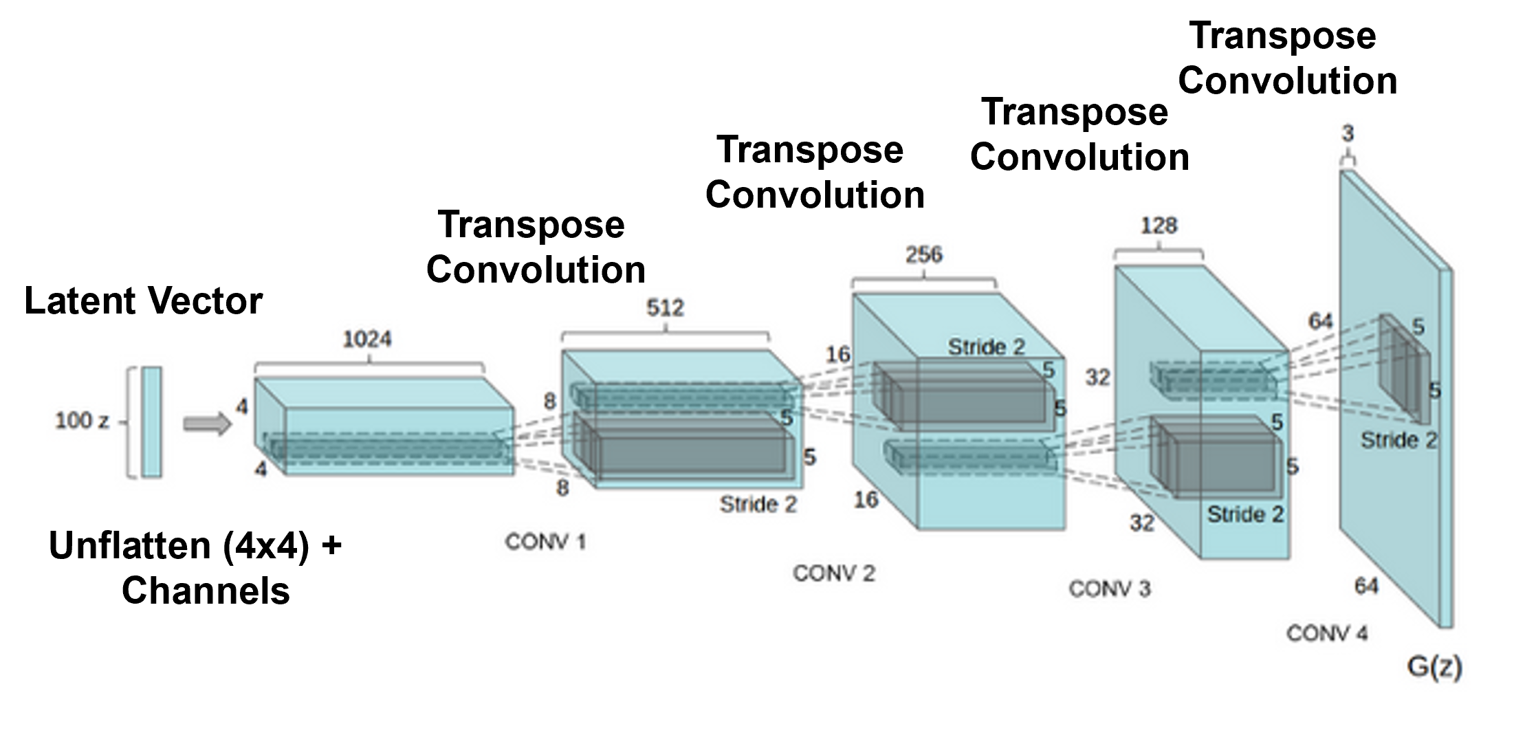
If we start with a convolutional neural network and we flip it, i.e., reverse the order of the operations,
we have a machine that maps from a 1D vector of values, to an image, i.e., we can generate fake images by randomly assigning latent values
to accomplish this instead of convolution operations with activation, we have transpose convolution operations with activation to move to the next feature map
recall we also perform non-linear activation at each feature map to prevent network collapse
But how do we train this flipped convolutional neural network to make good images?
we could take training images and score the difference between our generated fake images, for example, with a pixel-wise squared error (L2 norm)
but if we did this, our machine learning model would only learn how to make this image or a limited set of training images and that would not be useful
We want to make a diverse set of image realizations, that look and behave correctly. This is the simulation paradigm at the heart of geostatistics,
to learn more about the simulation paradigm from geostatistics, see my Simulation Chapter from my free, online e-book, Applied Geostatistics in Python.
Instead of a typically loss function, we apply a classification convolutional neural network to map from the image to a probability of a real image, i.e., our loss function is effectively a network that learns to score the loss during training.
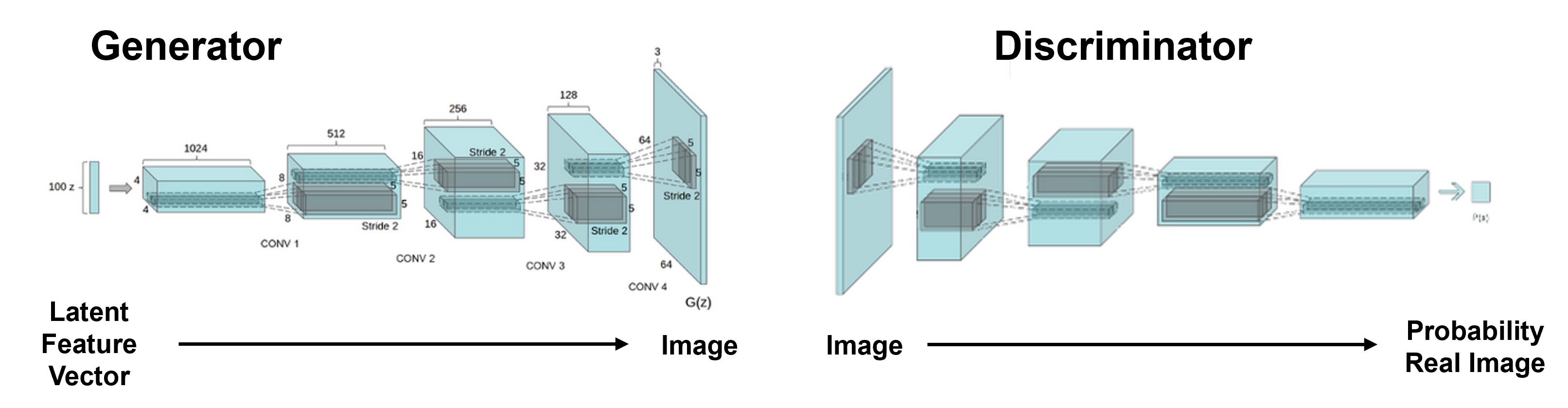
We have 2 neural networks in our GAN,
generator - flipped convolutional neural network that makes random fake images
discriminator - classification convolutional neural netwrok that calculates the probability that an image is real
Indirect, Adversarial Learning#
How do we train these two coupled networks? We call each network an agent and we train them competively, e.g., they compete while learning!
agent 1, Generator, is not trained to minimize an loss function with respect to training data (training image), no MSE!
instead the agent 1, Generator, is trained to fool agent 2, Discriminator
agent 2, Discriminator, is learning at the same time to tell the difference between the real training images and the fakes from agent 1, generator
Each agent has their own competitive goals,
Generator – make fakes that Discriminator classifies as real
Discriminator – correctly classify fake and real images
Note, the generator never sees the real images, but by learning to fool the discriminator learns to make images like the real training images.
The GAN loss function is stated as,
where,
\(\theta_D\) - parameters (weights, biases) of the discriminator
\(\theta_G\) - parameters of the generator
\(D_{\theta_D}(\cdot)\) - discriminator output, given the discriminator parameters \(\theta_D\) (probability input is real)
\(G_{\theta_G}(\mathbf{x})\) - output of the Generator output given latent input \(\mathbf{x}\)
\(\mathbf{y} \sim p_{\text{data}}\) - training images from the real image set
\(\mathbf{x} \sim p_{\mathbf{x}}\) - latent input sampled from known prior (e.g. uniform or normal)
\(\mathbb{E}[\cdot]\) - expectation over data (i.e., average over all samples)
\(\log D(\cdot)\) - log-likelihood that the discriminator assigns input as real
\(\log(1 - D(G(\cdot)))\) - log-likelihood that discriminator assigns fake to generator’s output
The discriminator wants to maximize,
tries to correctly predicts real training images as real, \(\log D(\mathbf{y}) \rightarrow 0.0\)
and to correctly predicts generated fake training images as not real, \(\log(1 - D(G(\mathbf{x}))) \rightarrow 0.0\)
The generator want to minimize,
tries to fool the discriminator, discriminator classifies fake training images as real, \(\log(1 - D(G(\mathbf{x}))) \rightarrow -\infty\)
To assist with understanding the GAN loss function and the system of competing agents, consider these end members,
Perfect Discriminator - if the discriminator is perfect,
all real training images are classified as real, \(D(\mathbf{y}) = 1\)
all fake images from the generator are classified as real, \(D(G(\mathbf{x})) = 0\)
\(\quad\) then the discriminator loss is,
\(\quad\) this sounds like good news, i.e., the generator will then improve to catch up with the discriminator, but what actually happens is,
generator receives no loss gradients, because the generators gradients,
\(\quad\) if \(D(G(z)) \to 0\), this derivative becomes zero, so training stalls and the generator doesn’t learn,
this is practically solved by substituting non-saturating generator loss for the generator,
\(\quad\) if \(D(G(z)) \to 0\), then \(\log D(G(z)) \to -\infty\), so the gradient becomes large, giving the generator a strong learning signal.
Perfect Generator - if the generator is perfect,
all fake images have the same distribution as the real training images, \(G(\mathbf{x}) \sim p_{\text{data}}\)
the best the discriminator can do is to assign a anive classification, \(D(\cdot) = 0.5\), for all fake and real training images
\(\quad\) then the loss is,
discriminator is maximally confused
this is a Nash equilibrium for the GAN, because no player can improve their outcome by unilaterally changing their strategy, assuming the other player’s strategy stays the same, generator is already making perfect images and discriminator can only guess naively, 50/50 real and fake.
Import Required Packages#
We will also need some standard packages. These should have been installed with Anaconda 3.
recall our goal is to build a convolutional neural network by-hand with only basic math and array operations, so we only need NumPy along with matplotlib for plotting.
%matplotlib inline
suppress_warnings = True                                      # toggle to supress warnings
import os                                                     # set working directory
import numpy as np                                            # arrays and matrix math
import matplotlib.pyplot as plt                               # for plotting
import matplotlib.patches as patches                          # fancy box around agents
from matplotlib.ticker import (MultipleLocator, AutoMinorLocator) # control of axes ticks
from matplotlib.ticker import FuncFormatter
import copy                                                   # deep copy dictionaries
import math
seed = 42
cmap = plt.cm.inferno                                         # default color bar, no bias and friendly for color vision defeciency
plt.rc('axes', axisbelow=True)                                # grid behind plotting elements
if suppress_warnings == True:
    import warnings                                           # supress any warnings for this demonstration
    warnings.filterwarnings('ignore')
seed = 42                                                     # random number seed for workflow repeatability
If you get a package import error, you may have to first install some of these packages. This can usually be accomplished by opening up a command window on Windows and then typing ‘python -m pip install [package-name]’. More assistance is available with the respective package docs.
Declare Functions#
Here’s the functions to make, train and visualize our generative adversarial network, including the steps,
make a simple set of synthetic data
initialize the weights in our generator and discriminator
apply our generator and discrimintor
calculate the error derivative and update the generator and discriminator weights and biases
Here’s a list of the functions,
generate_real_data - synthetic data generator
initialize_generator_weights - assign small random weights and bias for generator
initialize_discriminator_weights - assign small random weights and bias for discriminator
generator_forward - calculate a set of fake data with the generator given a set of latent values and the current weights and biases
discriminator_forward - calculate the probability of a real image over a set of images and return a 1D ndarray of probabilities
sigmoid - activation function to apply in the generator and discriminator
generator_gradients - compute generator gradients averaged over the batch
discriminator_gradients - compute generator gradients averaged over the batch
Here are the functions.
def sigmoid(x):                                               # sigmoid activation function
    return 1 / (1 + np.exp(-x))

def generate_real_data(batch_size, slope_range=(-0.4, -0.7), residual_std=0.02): # make a synthetic training image set
    """
    Generate real 3-node images with decreasing linear trend plus noise.
    Standardize each to have mean 0.5.
    Returns shape (batch_size, 3)
    """
    slopes = np.random.uniform(slope_range[0], slope_range[1], size=batch_size)
    base = np.array([1, 2, 3])  # node positions for linear trend
    data = np.zeros((batch_size, 3))
    for i in range(batch_size):
        trend = slopes[i] * base
        residual = np.random.normal(0, residual_std, size=3)
        sample = trend + residual
        sample += 0.5 - np.mean(sample)                       # standardize to mean 0.5
        data[i] = sample
    return data

def initialize_generator_weights():                           # initialize the generator weights and return as a dictionary
    # Small random weights and bias for generator
    return {
        'lambda_12': np.random.randn() * 0.1,
        'lambda_13': np.random.randn() * 0.1,
        'lambda_14': np.random.randn() * 0.1,
        'b': 0.0
    }

def generator_forward(L1_latent, weights,return_pre_activation=False): # given latent vector and generator weights return a set of fake images
    """
    L1_latent: ndarray shape (batch_size,)
    weights: dict with keys 'lambda_1_2', 'lambda_1_3', 'lambda_1_4', 'b'
    Returns output ndarray shape (batch_size, 3)
    """
    O2in = weights['lambda_12'] * L1_latent + weights['b']
    O3in = weights['lambda_13'] * L1_latent + weights['b']
    O4in = weights['lambda_14'] * L1_latent + weights['b']

    O2 = sigmoid(O2in)
    O3 = sigmoid(O3in)
    O4 = sigmoid(O4in)

    Oin = np.vstack([O2in, O3in, O4in]).T; O = np.vstack([O2, O3, O4]).T;

    if return_pre_activation:
        return np.vstack([O2in, O3in, O4in]).T, np.vstack([O2, O3, O4]).T # shape (batch_size, 3)
    else:
        return np.vstack([O2, O3, O4]).T # shape (batch_size, 3)

def initialize_discriminator_weights():                       # initialize the discriminator weights and return as a dictionary
    return {
        'lambda_58': np.random.randn() * 0.1,
        'lambda_68': np.random.randn() * 0.1,
        'lambda_78': np.random.randn() * 0.1,
        'c': 0.0
    }

def discriminator_forward(I5, I6, I7, weights):               # given a set of images return the discriminator probability of real image
    """
    Inputs: I5, I6, I7 shape (batch_size,)
    weights: dict with keys 'lambda_58', 'lambda_68', 'lambda_78', 'c'
    Returns probability ndarray shape (batch_size,)
    """
    dO8in = (weights['lambda_58'] * I5 +
         weights['lambda_68'] * I6 +
         weights['lambda_78'] * I7 +
         weights['c'])
    dO8 = sigmoid(dO8in)
    return dO8, dO8in

def discriminator_gradients(I5, I6, I7, y_true, weights):     # given set of images, true labels, and discriminator weights return the gradients
    """
    Compute discriminator gradients averaged over batch.
    y_true: labels (1 for real, 0 for fake), shape (batch_size,)
    """
    batch_size = y_true.shape[0]
    y_pred, z = discriminator_forward(I5, I6, I7, weights)
    dO8in = (y_pred - y_true)                                  # shape (batch_size,), note this solution integrates the sigmoid activation at O8

    grad_lambda_58 = np.mean(dO8in * I5)
    grad_lambda_68 = np.mean(dO8in * I6)
    grad_lambda_78 = np.mean(dO8in * I7)
    grad_c = np.mean(dO8in)

    return {
        'lambda_58': grad_lambda_58,
        'lambda_68': grad_lambda_68,
        'lambda_78': grad_lambda_78,
        'c': grad_c
    }

def generator_gradients(L1_latent, weights_g, weights_d):     # given latent vector, generator and discriminator weights return the gradients
    """
    Compute gradients of generator weights using discriminator feedback.
    L1_latent: shape (batch_size,)
    weights_g: generator weights dict
    weights_d: discriminator weights dict
    """
    batch_size = L1_latent.shape[0]

    #O = generator_forward(L1_latent, weights_g)               # generator outputs, shape (batch_size, 3)
    O_in, O = generator_forward(L1_latent, weights_g, return_pre_activation=True)

    O2_in, O3_in, O4_in = O_in[:, 0], O_in[:, 1], O_in[:, 2]
    O2, O3, O4 = O[:,0], O[:,1], O[:,2]
    I5, I6, I7 = O[:,0], O[:,1], O[:,2]

    y_pred, z = discriminator_forward(I5, I6, I7, weights_d)  # discriminator forward pass

    dO8in = y_pred - 1                                           # gradient of loss w.r.t discriminator logit for generator loss, shape (batch_size,)

    dO2 = dO8in * weights_d['lambda_58']                         # gradients w.r.t generator outputs
    dO3 = dO8in * weights_d['lambda_68']
    dO4 = dO8in * weights_d['lambda_78']

    dO2in = dO2 * O2 * (1 - O2)                                  # Backprop through generator sigmoid activation
    dO3in = dO3 * O3 * (1 - O3)
    dO4in = dO4 * O4 * (1 - O4)

    grad_lambda_12 = np.mean(dO2in * L1_latent)                 # gradients w.r.t generator weights and bias
    grad_lambda_13 = np.mean(dO3in * L1_latent)
    grad_lambda_14 = np.mean(dO4in * L1_latent)
    grad_b = np.mean(dO2in + dO3in + dO4in)

    return {
        'lambda_12': grad_lambda_12,
        'lambda_13': grad_lambda_13,
        'lambda_14': grad_lambda_14,
        'b': grad_b
    }

def fancybox(ax, xy, width, height, label="", edgecolor="black", text_color=None): # a dashed fancy box for the GAN plot
    """
    Draws a dashed, rounded rectangle on a given axes.

    Parameters:
    - ax: The matplotlib axes to draw on
    - xy: (x, y) tuple for bottom-left corner of the box
    - width: Width of the box
    - height: Height of the box
    - label: Optional label text to display centered above the box
    - edgecolor: Border color of the box
    - text_color: Color of the label text (defaults to edgecolor)
    """
    if text_color is None:
        text_color = edgecolor

    box = patches.FancyBboxPatch(                             # draw box
        xy,
        width,
        height,
        boxstyle="round,pad=0.02",
        linewidth=2,
        edgecolor=edgecolor,
        facecolor="none",
        linestyle='--'
    )
    ax.add_patch(box)

    x_center = xy[0] + width / 2                              # add label text above the box
    y_top = xy[1] + height + 0.02
    ax.text(x_center, y_top + 0.02, label, ha='center', va='bottom', fontsize=16, color=text_color)

def add_grid2():                                              # add grid lines
    plt.gca().grid(True, which='major',linewidth = 1.0); plt.gca().grid(True, which='minor',linewidth = 0.2) # add y grids
    plt.gca().tick_params(which='major',length=7); plt.gca().tick_params(which='minor', length=4)
    plt.gca().xaxis.set_minor_locator(AutoMinorLocator()); plt.gca().yaxis.set_minor_locator(AutoMinorLocator()) # turn on minor ticks
Set the Working Directory#
I always like to do this so I don’t lose files and to simplify subsequent read and writes (avoid including the full address each time).
#os.chdir("c:/PGE383") # set the working directory
Visualize the Generative Adversarial Network#
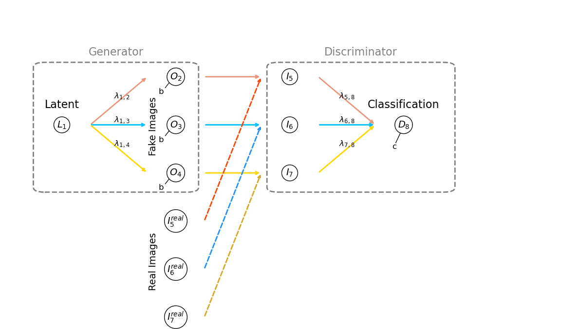
We are implementing a minimal Generative Adversarial Network (GAN) with the 2 agents,
Generator - that produces 3-node outputs (like tiny 1D images) from a single latent input
Discriminator - that evaluates these outputs to distinguish between real and fake samples.
Now let’s define the parts of the Generator,
Latent Node - \(L_1\), a single random value with uniform distribution, \(U[0.4,1.0]\). Note we set the minimum as 0.4 to stay away from 0.0 or negative values as these would remove the slope or flip the slope of the fakes.
Generator Weights - \(\lambda_{1,2}\), \(\lambda_{1,3}\) and \(\lambda_{1,4}\) for the connections from latent to each of the output nodes. This is the simplest possible tranpose convolution, with a kernel size is 3, output nodes is 3 and latent node is 1, so the kernel does not translate. I did this to greatly simplify the book keeping, but the concepts could be extended to a more realistic convolution / tranpose convolution architectures for more realistic images sizes problem.
Generator Bias - \(b\), a single, constant bias over the output layer (output image), the nodes, \(O_2\), \(O_3\), and \(O_4\)
Generator Output Nodes - \(O_2\), \(O_3\), and \(O_4\), the single and last feature map in our very simple generator; therefore, the output a 1D image with 3 nodes or pixels that are passed to the Discriminator input nodes, \(I_5\), \(I_6\), and \(I_7\)
Discriminator Input Nodes - \(I_5\), \(I_6\), and \(I_7\), that receive the real images or the fake images from the generator output nodes, \(O_2\), \(O_3\), \(O_4\)
Discriminator Weights - \(\lambda_{5,8}\), \(\lambda_{6,8}\), and \(\lambda_{7,8}\) for the connections from input nodes (input image) to the output (descision) node, \(D_8\)
Discriminator Bias - \(c\), bias applied at the output (descision) node, \(D_8\)
Now let’s visualize this very simple generative adversarial network.
colors = ['darksalmon','deepskyblue','gold']                  # line colors for latent to fake to probability flow
colors_real = ['orangered','dodgerblue','goldenrod']          # line colors for real image to probability flow

def draw_gan_architecture_full():                             # function to draw the GAN demonstrated in this workflow
    fig, ax = plt.subplots(figsize=(12, 7))

    ax.text(0.1, 0.5, r"$L_1$", fontsize=14, ha='center', va='center', # generator latent node
            bbox=dict(boxstyle="circle", fc="white", ec="black"))

    gen_outputs = [                                           # generator output nodes locations and labels
        (0.3, 0.7, r"$O_2$", r"$\lambda_{1,2}$"),
        (0.3, 0.5, r"$O_3$", r"$\lambda_{1,3}$"),
        (0.3, 0.3, r"$O_4$", r"$\lambda_{1,4}$")
    ]
    for i, (x, y, label, weight) in enumerate(gen_outputs):   # generator output node labels
        ax.text(x, y, label, fontsize=14, ha='center', va='center',
                bbox=dict(boxstyle="circle", fc="white", ec="black"))
        ax.annotate("", xy=(x - 0.05, y), xytext=(0.15, 0.5),   # generator output node connections
                    arrowprops=dict(arrowstyle="->", lw=2, color=colors[i]))
        ax.text((x + 0.11) / 2, (y + 0.5) / 2, weight, fontsize=12, ha='center', va='bottom')

    disc_inputs = [                                           # discriminator input nodes locations and labels
        (0.5, 0.7, r"$I_5$", r"$\lambda_{5,8}$"),
        (0.5, 0.5, r"$I_6$", r"$\lambda_{6,8}$"),
        (0.5, 0.3, r"$I_7$", r"$\lambda_{7,8}$")
    ]
    for i, (x, y, label, _) in enumerate(disc_inputs):        # discriminator input node labels
        ax.text(x, y, label, fontsize=14, ha='center', va='center',
                bbox=dict(boxstyle="circle", fc="white", ec="black"))
        ax.annotate("", xy=(x - 0.05, y), xytext=(0.35, gen_outputs[i][1]), # discriminator input node connections
                    arrowprops=dict(arrowstyle="->", lw=2, color=colors[i]))

    ax.text(0.7, 0.5, r"$D_8$", fontsize=14, ha='center', va='center', # discriminator decision node label
            bbox=dict(boxstyle="circle", fc="white", ec="black"))
    for i, (x, y, _, weight) in enumerate(disc_inputs):
        ax.annotate("",xy=(0.65, 0.5), xytext=(x + 0.05, y),  # discriminator output node connections
                    arrowprops=dict(arrowstyle="->", lw=2, color=colors[i]))
        ax.text((x + 0.7) / 2, (y + 0.5) / 2, weight, fontsize=12, ha='center', va='bottom')

    real_inputs = [                                           # real data path below generator
        (0.3, 0.1, r"$I_5^{real}$"),
        (0.3, -0.1, r"$I_6^{real}$"),
        (0.3, -0.3, r"$I_7^{real}$")
    ]
    for i, (x, y, label) in enumerate(real_inputs):
        ax.text(x, y, label, fontsize=14, ha='center', va='center', # label real data node labels
                bbox=dict(boxstyle="circle", fc="white", ec="black"))
        ax.annotate("",                                       # arrow to discriminator inputs
                    xy=(disc_inputs[i][0] - 0.05, disc_inputs[i][1]),
                    xytext=(x + 0.05, y),
                    arrowprops=dict(arrowstyle="->", lw=2, color=colors_real[i], linestyle="--"))

    ax.text(0.1, 0.57, "Latent", fontsize=16, ha='center')    # GAN part labels
    ax.text(0.7, 0.57, "Classification", fontsize=16, ha='center')
    ax.text(0.26, -0.18, "Real Images", fontsize=14, ha='center', color="black",rotation=90.0)
    ax.text(0.26, 0.38, "Fake Images", fontsize=14, ha='center', color="black",rotation=90.0)

    fancybox(ax, xy=(0.07, 0.24), width=0.25, height=0.5, label="Generator", edgecolor="grey") # fancy boxes around generator and discriminator
    fancybox(ax, xy=(0.48, 0.24), width=0.29, height=0.5, label="Discriminator", edgecolor="grey")

    ax.text(0.68,0.4,'c',fontsize=12,color='black')           # draw the biases in O2, O3, O4 and D8
    ax.annotate("", xy=(0.695, 0.47), xytext=(0.685, 0.42),arrowprops=dict(arrowstyle="-", color="black", lw=1))
    ax.text(0.27,0.63,'b',fontsize=12,color='black')
    ax.annotate("", xy=(0.28, 0.65), xytext=(0.29, 0.68),arrowprops=dict(arrowstyle="-", color="black", lw=1))
    ax.text(0.27,0.43,'b',fontsize=12,color='black')
    ax.annotate("", xy=(0.28, 0.45), xytext=(0.29, 0.48),arrowprops=dict(arrowstyle="-", color="black", lw=1))
    ax.text(0.27,0.23,'b',fontsize=12,color='black')
    ax.annotate("", xy=(0.28, 0.25), xytext=(0.29, 0.28),arrowprops=dict(arrowstyle="-", color="black", lw=1))
    ax.axis('off')
    plt.tight_layout()
    plt.show()

draw_gan_architecture_full()                                  # draw the GAN
Just a couple more comments about my network nomenclature. My goal is to maximize simplicity and clarity,
Sigmoid Activation#
For reference, let’s visualize the sigmoid activation function,
activation - the non-linear transformation, this is the sigmoid activation
activation derrivative - essential for back propogation
note, for convenience the derrivative of the sigmoid activation function with respect to the input is posed for the output.
as we back-propogate backwards over the activation function we can us the output to step back through the activated network node
amin = -5.0; amax = 5.0

input = np.linspace(amin,amax,100); output = 1.0/(1.0 + np.exp(-1*np.linspace(amin,amax,100))); derriv = output * (1 - output)

plt.subplot(111)
plt.plot(input,output,color='forestgreen',lw=2,label='Activation'); add_grid2(); plt.xlabel('Input'); plt.ylabel('Output')
plt.plot(input,derriv,color='deepskyblue',lw=2,label='Derrivative'); add_grid2(); plt.xlabel('Input'); plt.ylabel('Output')
plt.title('Sigmoid Activation'); plt.legend(loc='upper left'); plt.xlim([amin,amax])

plt.subplots_adjust(left=0.0, bottom=0.0, right=2.0, top=1.1, wspace=0.2, hspace=0.2); plt.show()
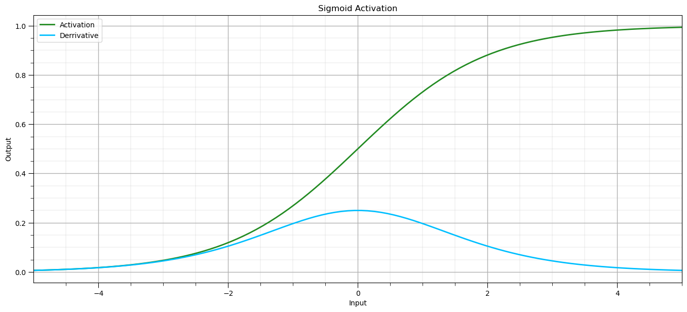
Let’s make some observations about the sigmoid activation and its derrivative,
sigmoid outputs - are bounded (0,1) approaching both limits asymptotically
vanishing gradients - as the
Generator Forward Pass#
First, let’s walk through the generator to go from a latent value to a fake image. The generator takes a latent input,
recall, our simple generator has only one layer \(L1\), with only 3 outputs, \(O_2\), \(O_3\), and \(O_4\), representing the fake image.
Then latent value, \(L_1\), is passed through the transpose convolution kernel to the output,
our transpose convolution kernel has a size of 3, the same size as our output, so we don’t see it translate it, resulting in greatly simplified book keeping!
the tranpose convolution kernel weights are \(\lambda_{1,2}\), \(\lambda_{1,3}\), and \(\lambda_{1,4}\)
We apply the sigmoid activation in each of the output nodes
Each output is computed by applying a linear transformation followed by a sigmoid activation, \(\sigma\),
where,
\(\lambda_{1,j}\) - are the transpose convolution kernel weights
\(b\) - is the shared bias, single bias term for the output layer
We can also write the generator forward pass in matrix notation as,
where the sigmoid activation is applied element-wise.
Discriminator Forward Pass#
Now let’s walk-through the discriminator, going from an image, real or fake, to a probability of real. The discriminator receives the image, over 3 input nodes, \(I_5\), \(I_6\), and \(I_7\). In the case of a fake image,
and in the case of a real image,
Since we have only 1 layer and the convolution kernel is 3 with an input of 3 once again there is no translation!
we just take input image, \(I_5\), \(I_6\), and \(I_7\), and apply the convolutional kernel weights, \(\lambda_{5,8}\), \(\lambda_{6,8}\), and \(\lambda_{7,8}\), and add the bias term, \(c\),
where,
\(\lambda_{i,8}\) are the convolutional kernel weights to go from input image to next feature map, only 1 value, our output probability
\(c\) is the bias term
\(\sigma(x) = \dfrac{1}{1 + e^{-x}}\) is the sigmoid activation function
\(D_8 \in [0, 1]\) represents the probability assigned by the discriminator that the input is real (i.e. not a fake from the generator).
We can also write the discriminator forward pass in matrix notation as,
where,
\(\lambda_{5,8}, \lambda_{6,8}, \lambda_{7,8}\) are scalar weights
\(I_5, I_6, I_7\) are the input values (i.e., outputs of the generator, \(O_2, O_3, O_4\))
\(c\) is the bias term
\(\sigma(x) = \dfrac{1}{1 + e^{-x}}\) is the sigmoid function
Discriminator Loss#
Binary cross-entropy is a loss function used for binary classification tasks where the output is a probability between 0 and 1, and the target label is either 0 or 1.
Prediction (model output) - \(\hat{y} \in (0, 1)\), the output of \(D_8\), the discriminator’s classification, probability that the image is real
True label (ground truth) - \(y \in \{0, 1\}\), 0 if the image is from the generator, fake, and 1 if the image is from the real training data
Now we can define the binary cross-entropy loss as,
now we can further specify,
\(\log(\hat{y})\) is the log-likelihood of the positive prediction
\(log(1 - \hat{y})\) is the log-likelihood of the negative prediction
how does binary cross-entropy behave?
if \(y = 1\) (real image), then:
if \(y = 0\) (fake image from the generator), then:
We can summarize as,
the loss is low when the model’s prediction \(\hat{y}\) is close to the true label, low probability of real for a fake image and high probability of real for a real image
the loss becomes very large if the model is confident and wrong, due to the logarithm, i.e., very low probability or real for a real image and very high probability of real for a fake image
the sigmoid activation ensures that the output, \(\hat{y}\) is a valid probability
Discriminator Loss Derivative#
To perform backpropagation we need to calculate the loss derivative. Let’s do this for the input of the activation function as our output node, \(D_8\),
define \(z\) as the input for the sigmoid activation as output node, \(D_8\).
as you see we do this because it results in a very simple, efficient result.
recall, the sigmoid function,
We will use the chain rule, so we only need to solve the parts,
\(\frac{d\mathcal{L}}{d\hat{y}}\) - partial derivative of binary cross-entropy loss given the discriminator output \(\hat{y}\) (\(D_8\))
\(\frac{d\hat{y}}{dz}\) - partial derivative of the discriminator output \(\hat{y}\) (\(D_8\)) given the sigmoid activation input
Now we can solve the first part, partial derivative of loss with respect to the discriminator output, \(\hat{y}\)
now we can solve the second part, the partial derivative of the discriminator output \(\hat{y}\) (\(D_8\)) given the sigmoid activation input, it is just the sigmoid derivative,
and we can combine these by the chain rule as,
We are almost there, we only need to simplify the result, first we distribute, \(\hat{y}(1 - \hat{y})\),
and then simplify it further,
I said this would get simple! Our partial derivative of our loss with respect to the input to the output node sigmoid activation function, \(z\), is,
This result shows the gradient is just the error — the difference between predicted and true values.
Now we can make this simple interpretation,
if \(\hat{y} > y\), the model overestimates \(\rightarrow\) gradient is positive \(\rightarrow\) lower prediction by moving in the negative gradient
if \(\hat{y} < y\), the model underestimates \(\rightarrow\) gradient is negative \(\rightarrow\) increase prediction by moving in the negative gradient
I know that a title this section “Discriminator Loss Derivative”, but excuse me for performing just a little bit of backpropagation (to before sigmoid activation).
next we carry on with back propagation to the discriminator weights and biases
Discriminator Back Propagation#
For compact notation, let’s use matrix notation and define the input to the \(D_8\) activation, \(z\), as,
Now we can extend our use of the chain rule to,
So for each of our discriminator weights, \(\lambda_{5,8}\), \(\lambda_{6,8}\), and \(\lambda_{7,8}\) we have,
and for the bias, \(c\), we calculate the next component for the chain rule as,
so we have,
The backpropagation for our very simple discriminator is quite simple, we can summarize for the weights,
and for the bias,
Let’s write these out for all of our discriminators parameters, $\( \begin{aligned} \frac{d\mathcal{L}}{d\lambda_{5,8}} &= (\hat{y} - y) \cdot I_5 \\ \frac{d\mathcal{L}}{d\lambda_{6,8}} &= (\hat{y} - y) \cdot I_6 \\ \frac{d\mathcal{L}}{d\lambda_{7,8}} &= (\hat{y} - y) \cdot I_7 \\ \frac{d\mathcal{L}}{dc} &= \hat{y} - y \end{aligned} \)$
Generator Loss Derivative and Back Propagation Through the Discriminator#
Recall that the goal of the generator is to make fake images the discriminator assigns as a high probability of a real image, i.e., to fool the discriminator
the generator produces a fake image,
\(\quad\) where ( z ) is a latent vector (e.g., sampled from Uniform[0.4, 1]).
the discriminator evaluates this fake sample and returns:
Now we can calculate the binary cross-entropy for the generator as,
where,
\(\hat{y} = D(G(z))\), the discriminator’s evaluation of the generator’s fake image, \(z\)
\(\hat{y}\) is the probability assigned by the discriminator to the fake being real
This is equivalent to cross-entropy with target label \(y = 1\), note here we do a trick, from the generator’s perspective it’s images are real, so we are using \(y=1\), i.e., real images for the fake images!
You may get confused if you look at the original GAN loss above, this is called the non-saturating generator loss.
Loss Type |
Expression |
Comment |
|---|---|---|
Original GAN |
\(\mathbb{E}[\log(1 - D(G(z)))]\) |
Theoretical, can cause vanishing gradients |
Non-saturating |
\(-\mathbb{E}[\log(D(G(z)))]\) |
Practical, stronger gradients, commonly used |
so instead of minimizing the original generator loss we are maximizing the non-saturating generator loss.
Let’s show how to back propagate through the entire discriminator with the chain rule.
we want the generator loss gradient with respect generator output,
Given \(\tilde{\mathbf{x}} = G(z)\), our fake image, we want the partial derivative of the loss given our fake image,
and by the chain rule,
This is how the discriminator’s belief \(\hat{y}\) about “fakeness” changes with changes in \(\tilde{\mathbf{x}}\) the fake image.
Now we are ready to back propagate the generator loss through the discriminator, let’s start with our generator loss (from above),
and when we perform the partial derivative,
Now, recall the discriminator’s forward pass is,
so we can calculate the partial derivative of the discriminator’s output with respect to the generator’s fake image as,
now we combine these with the chain rule as,
The gradient of the generator’s loss with respect to the output image \(\tilde{\mathbf{x}}\) is,
We can add some interpretations of this result,
when \(\hat{y}\) is close to 0 \(\rightarrow\) discriminator easily spots fake \(\rightarrow\) large gradient \(\rightarrow\) generator updates more.
when \(\hat{y}\) is close to 1 \(\rightarrow\) generator is fooling the discriminator \(\rightarrow\) gradient is small.
This guides the generator to tweak its output to increase \(\hat{y}\) — i.e., fool the discriminator.
To further clarify, for our example let’s compute how the discriminator’s output \(\hat{y}\) changes with respect to the generator outputs \(O_5, O_6, O_7\), instead of the \(w\) vector notation used above.
if we apply the chain rule we get,
\(\quad\) for each of the components we have,
\(\quad\) substituting in the chain rule we have,
Backpropagation Through Generator to Weights and Bias#
We now propagate through the generators sigmoid activation in each of the output nodes,
\(O_i = \sigma(z_i)\), where \(z_i\) is the input for the output nodes, pre-activation, and \(O_i\) is output for the output nodes, post-activation
We Apply chain rule,
Recall,
so we can calculate the generator’s weights partial derivatives as,
and the generator’s bias partial derivative as,
Now we can put this all together with the chain rule, the partial derivatives of the generator loss with respect to the generator weights are,
and the partial derivative of the generator loss with respect to the generator bias is,
For clarity, let’s write this out for each of our generator’s weights,
and for our generator’s bias,
Let’s make some interpretations,
the generator’s weights and bias gradients scale with how much the discriminator is fooled (\(1 - \hat{y}\))
the generator learns to tweak \(\lambda_{1,i}\) and \(b\) to push the fake images, \(O_5\), \(O_6\) and \(O_7\) in directions that increase \(\hat{y}\)
this flow of error gives the generator a signal to fool the discriminator more effectively without ever seeing a real image!
Simple GAN Training Workflow#
We start with initialization of the generator and discriminator weights and bias and setting the training hyperparameters.
Generate the Synthethic, “Real Images” for training
sample \(N\) real 3-node, 1D images \(\mathbf{I} = \{(I_{5,i}, I_{6,i}, I_{7,i})\}_{i=1}^N\)
use the synthetic training data function:
Initialize generator weights and bias - the weights,
\(\quad\) and the bias,
Initialize discriminator weights and bias - the weights,
\(\quad\) and the bias,
Set model training hyperparameters - this includes,
Learning Rates - for the generator, \(\eta_G\), and discriminator, \(\eta_D\)
Batch Size - in this example we are assuming batch size equal to the number of real images
Epochs - number of training iterations
Train the discriminator
combine real and fake inputs into a batch of size \(2N\) and inlcude labels \(y_i = 1\) for real, \(y_i = 0\) for fake
compute discriminator outputs \(\hat{y}_i = D(I_{5,i}, I_{6,i}, I_{7,i})\)
calculate discriminator loss and gradients using:
update discriminator weights and bias:
Train the generator
Compute generator output fake images and pass to the discriminator to evaluate the outputs on these fakes, \(D_8\) same as \(y\)
Calculate generator loss gradients using,
Update generator weights and bias,
Repeat Until Convergence - or stop criteria is met, such as maximum number of training epochs, return to step 5.
Here a summary of the training loop,
Generate real data batch
Generate fake data batch
Update discriminator to better distinguish real/fake
Update generator to fool discriminator
Repeat
This adversarial training loop lets the generator learn to create data mimicking the real distribution, and the discriminator improve in spotting fakes.
def train_gan(epochs=1000,batch_size=32,lr_g=0.1,lr_d=0.1,verbose=True): # function for training the GAN
weights_epoch_list = []; weights_g_list = []
# Initialize weights
weights_g = initialize_generator_weights()
weights_d = initialize_discriminator_weights()
# Tracking losses
generator_losses = []
discriminator_losses = []
real_images = generate_real_data(batch_size) # one set of images
for epoch in range(epochs):
# Step 1: Generate real data
I5_real, I6_real, I7_real = real_images[:,0], real_images[:,1], real_images[:,2]
y_real = np.ones(batch_size)
# Step 2: Generate fake data
L1_fake = np.random.uniform(0.4, 1, batch_size)
fake_images = generator_forward(L1_fake, weights_g,return_pre_activation=False)
I5_fake, I6_fake, I7_fake = fake_images[:,0], fake_images[:,1], fake_images[:,2]
y_fake = np.zeros(batch_size)
# Combine for discriminator training
I5_combined = np.concatenate([I5_real, I5_fake])
I6_combined = np.concatenate([I6_real, I6_fake])
I7_combined = np.concatenate([I7_real, I7_fake])
y_combined = np.concatenate([y_real, y_fake])
# Step 3: Train discriminator
grads_d = discriminator_gradients(I5_combined, I6_combined, I7_combined, y_combined, weights_d)
for key in weights_d:
weights_d[key] -= lr_d * grads_d[key]
# Step 4: Train generator
L1_gen = np.random.uniform(0.4, 1, batch_size)
grads_g = generator_gradients(L1_gen, weights_g, weights_d)
for key in weights_g:
weights_g[key] -= lr_g * grads_g[key]
# if epoch in [1000,2500,5000]: # save the weights to visualize model improvement over epochs
# weights_g_list.append(weights_g)
# Step 5: Calculate and store losses
y_pred_real, _ = discriminator_forward(I5_real, I6_real, I7_real, weights_d)
y_pred_fake, _ = discriminator_forward(I5_fake, I6_fake, I7_fake, weights_d)
loss_d_real = -np.mean(np.log(y_pred_real + 1e-8))
loss_d_fake = -np.mean(np.log(1 - y_pred_fake + 1e-8))
loss_d = loss_d_real + loss_d_fake
discriminator_losses.append(loss_d)
y_pred_gen, _ = discriminator_forward(*generator_forward(L1_gen, weights_g).T, weights_d)
loss_g = -np.mean(np.log(y_pred_gen + 1e-8))
generator_losses.append(loss_g)
# Print progress
if verbose and (epoch % 5000 == 0 or epoch == epochs - 1):
weights_epoch_list.append(epoch)
weights_g_list.append(copy.deepcopy(weights_g))
print(f"Epoch {epoch}: D_loss = {loss_d:.4f}, G_loss = {loss_g:.4f}")
# # Final output
# print("\nTraining complete.\nFinal Generator Weights:")
# for k, v in weights_g.items():
# print(f" {k}: {v:.4f}")
# print("\nFinal Discriminator Weights:")
# for k, v in weights_d.items():
# print(f" {k}: {v:.4f}")
return weights_g, weights_d, generator_losses, discriminator_losses, real_images, weights_g_list, weights_epoch_list
np.random.seed(seed=seed)
epochs = 50000
batch_size = 32
final_weights_g, final_weights_d, loss_g, loss_d, real_images, weights_g_list, weights_epoch_list = train_gan(epochs=epochs, batch_size=batch_size, lr_g=0.001, lr_d=0.001)
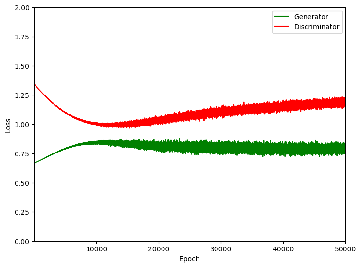
plt.plot(np.arange(1,epochs+1,1),loss_g,color='green',label='Generator')
plt.plot(np.arange(1,epochs+1,1),loss_d,color='red',label='Discriminator')
plt.xlim(1,epochs); plt.ylim(0,2.0); plt.ylabel('Loss'); plt.xlabel('Epoch'); plt.legend(loc='upper right')
plt.subplots_adjust(left=0.0, bottom=0.0, right=1.0, top=1.0, wspace=0.2, hspace=0.2); plt.show()
Epoch 0: D_loss = 1.3433, G_loss = 0.6666
Epoch 5000: D_loss = 1.0994, G_loss = 0.7903
Epoch 10000: D_loss = 1.0035, G_loss = 0.8478
Epoch 15000: D_loss = 0.9899, G_loss = 0.8271
Epoch 20000: D_loss = 1.0441, G_loss = 0.8124
Epoch 25000: D_loss = 1.0621, G_loss = 0.8129
Epoch 30000: D_loss = 1.1218, G_loss = 0.8277
Epoch 35000: D_loss = 1.1224, G_loss = 0.8411
Epoch 40000: D_loss = 1.1631, G_loss = 0.7914
Epoch 45000: D_loss = 1.1779, G_loss = 0.7685
Epoch 49999: D_loss = 1.1607, G_loss = 0.7617
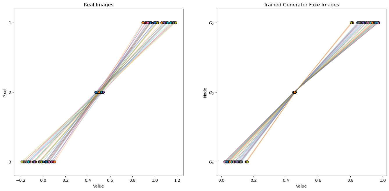
Visualize Real Images and Trained Generator Fake Images#
Let’s check a set of fake images from our trained generator against the real images.
recall the generator never saw these images, the discriminator saw the real and fake images and told the generator how good or bad were the generator’s fake images.
L1_test = np.random.uniform(0.4, 1, batch_size)
trained_fake = generator_forward(L1_test, weights_g_list[-1])
untrained_fake = generator_forward(L1_test, weights_g_list[0])

plt.subplot(121)
for i in range(0,batch_size):
    plt.plot(real_images[i],np.arange(1,4,1),alpha=0.3)
    plt.scatter(real_images[i],np.arange(1,4,1),edgecolor='black',zorder=10)
    plt.title('Real Images'); plt.xlabel('Value'); plt.ylabel('Node')
    plt.ylabel('Pixel'); plt.yticks([1, 2, 3]); plt.ylim([3.2,0.8])

plt.subplot(122)
for i in range(0,batch_size):
    plt.plot(trained_fake[i],np.arange(1,4,1),alpha=0.3)
    plt.scatter(trained_fake[i],np.arange(1,4,1),edgecolor='black',zorder=10)
    plt.title('Trained Generator Fake Images'); plt.xlabel('Value'); plt.ylabel('Node')
    plt.yticks([1, 2, 3], [r'$O_2$', r'$O_3$', r'$O_4$']); plt.ylim([3.2,0.8])

plt.subplots_adjust(left=0.0, bottom=0.0, right=2.0, top=1.2, wspace=0.2, hspace=0.2); plt.show()
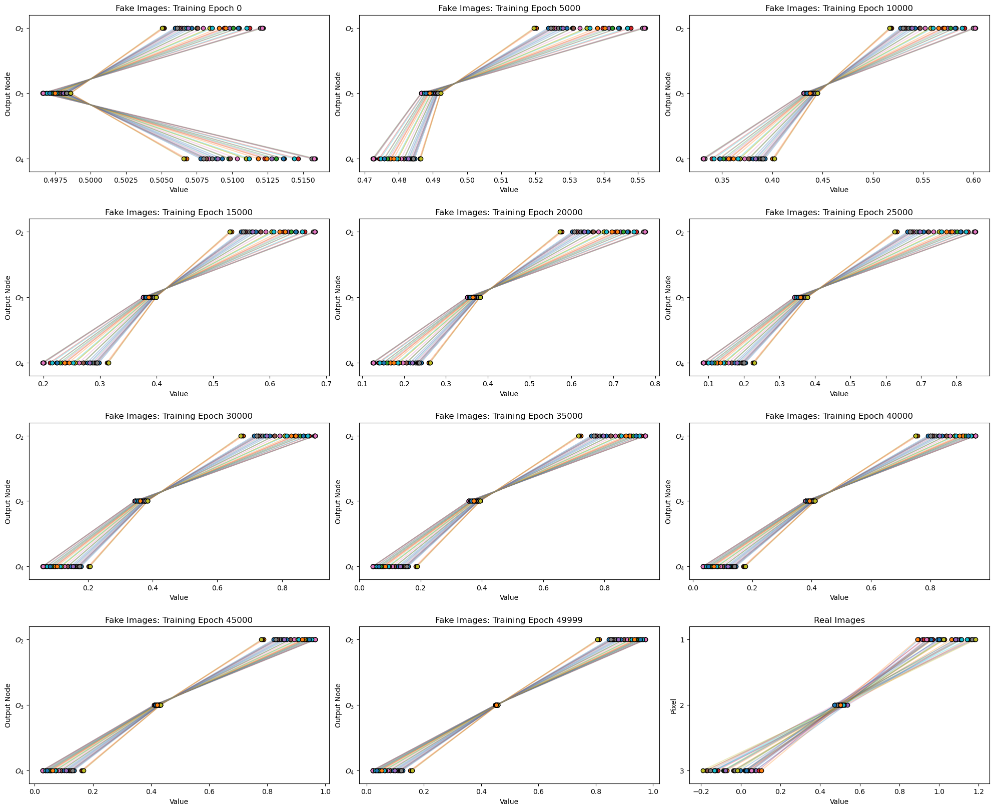
Visualize Real Images and Generator Fake Images Over Training Epochs#
It is interesting to see how our generator’s fake images evolve over the training epochs.
as first the fake images are random due to the random initialization of the generator’s weights and bias
as the training proceeds the generator learns to improve the fake images.
I include the real images at the end for comparison.
for i,weights_g in enumerate(weights_g_list):
    fake = generator_forward(L1_test, weights_g_list[i])
    plt.subplot(4,3,i+1)
    for j in range(0,batch_size):
        plt.plot(fake[j],np.arange(1,4,1),alpha=0.3)
        plt.scatter(fake[j],np.arange(1,4,1),edgecolor='black',zorder=10)
    plt.title('Fake Images: Training Epoch ' + str(weights_epoch_list[i])); plt.xlabel('Value'); plt.ylabel('Output Node')
    plt.yticks([1, 2, 3], [r'$O_2$', r'$O_3$', r'$O_4$']); plt.ylim([3.2,0.8])

plt.subplot(4,3,12)
for i in range(0,batch_size):
    plt.plot(real_images[i],np.arange(1,4,1),alpha=0.3)
    plt.scatter(real_images[i],np.arange(1,4,1),edgecolor='black',zorder=10)
    plt.title('Real Images'); plt.xlabel('Value'); plt.ylabel('Pixel'); plt.yticks([1, 2, 3]); plt.ylim([3.2,0.8])

plt.subplots_adjust(left=0.0, bottom=0.0, right=3.0, top=3.2, wspace=0.1, hspace=0.3); plt.show()
Comments#
This was a basic treatment of generative adversarial networks. Much more could be done and discussed, I have many more resources. Check out my shared resource inventory and the YouTube lecture links at the start of this chapter with resource links in the videos’ descriptions.
I hope this is helpful,
Michael
About the Author#

Michael Pyrcz is a professor in the Cockrell School of Engineering, and the Jackson School of Geosciences, at The University of Texas at Austin, where he researches and teaches subsurface, spatial data analytics, geostatistics, and machine learning. Michael is also,
the principal investigator of the Energy Analytics freshmen research initiative and a core faculty in the Machine Learn Laboratory in the College of Natural Sciences, The University of Texas at Austin
an associate editor for Computers and Geosciences, and a board member for Mathematical Geosciences, the International Association for Mathematical Geosciences.
Michael has written over 70 peer-reviewed publications, a Python package for spatial data analytics, co-authored a textbook on spatial data analytics, Geostatistical Reservoir Modeling and author of two recently released e-books, Applied Geostatistics in Python: a Hands-on Guide with GeostatsPy and Applied Machine Learning in Python: a Hands-on Guide with Code.
All of Michael’s university lectures are available on his YouTube Channel with links to 100s of Python interactive dashboards and well-documented workflows in over 40 repositories on his GitHub account, to support any interested students and working professionals with evergreen content. To find out more about Michael’s work and shared educational resources visit his Website.
Want to Work Together?#
I hope this content is helpful to those that want to learn more about subsurface modeling, data analytics and machine learning. Students and working professionals are welcome to participate.
Want to invite me to visit your company for training, mentoring, project review, workflow design and / or consulting? I’d be happy to drop by and work with you!
Interested in partnering, supporting my graduate student research or my Subsurface Data Analytics and Machine Learning consortium (co-PI is Professor John Foster)? My research combines data analytics, stochastic modeling and machine learning theory with practice to develop novel methods and workflows to add value. We are solving challenging subsurface problems!
I can be reached at mpyrcz@austin.utexas.edu.
I’m always happy to discuss,
Michael
Michael Pyrcz, Ph.D., P.Eng. Professor, Cockrell School of Engineering and The Jackson School of Geosciences, The University of Texas at Austin
More Resources Available at: Twitter | GitHub | Website | GoogleScholar | Geostatistics Book | YouTube | Applied Geostats in Python e-book | Applied Machine Learning in Python e-book | LinkedIn
Comments on Network Nomenclature#
Network Nodes and Connections - I choose to use unique numbers for all nodes, \(L_1\), \(O_2\), \(O_3\), \(\ldots\) instead of \(L_1\), \(O_1\), \(O_2\), \(\ldots\) to simplify the notation for the weights; therefore, when I say \(\lambda_{5,8}\) you know exactly where this weight is applied in the network.
Node Outputs - I use the node label to also describe the output from the node, for example \(O_2\) is a node in the generator’s output layer and also the signal or value output from that node.
Pre- and Post-activation - at our nodes \(O_2\), \(O_3\), \(O_4\), and \(D_8\) we have the node input before activation and the node output after activation, I use the notation \(O_{2_{in}}\), \(O_{3_{in}}\), \(O_{4_{in}}\) and \(D_{8_{in}}\) for the pre-activation input and \(O_2\), \(O_3\), \(O_4\), and \(D_8\) for the post-activation node output. This is important because with back propagation we have to step through the nodes, going from post-activation to pre-activation.
Latent - while publications often use \(z\) notation for the latent values, to be consistent with my notion above, I use \(L_1\) for the latent value, i.e., the output from my latent node, \(L_1\).
Now let’s walk-through all the parts of our example GAN and show all the math.