

Synthetic Datasets#
Michael J. Pyrcz, Professor, The University of Texas at Austin
Twitter | GitHub | Website | GoogleScholar | Geostatistics Book | YouTube | Applied Geostats in Python e-book | Applied Machine Learning in Python e-book | LinkedIn
Chapter of e-book “Applied Machine Learning in Python: a Hands-on Guide with Code”.
Cite this e-Book as:
Pyrcz, M.J., 2024, Applied Machine Learning in Python: A Hands-on Guide with Code [e-book]. Zenodo. doi:10.5281/zenodo.15169138 ![]()
The workflows in this book and more are available here:
Cite the MachineLearningDemos GitHub Repository as:
Pyrcz, M.J., 2024, MachineLearningDemos: Python Machine Learning Demonstration Workflows Repository (0.0.3) [Software]. Zenodo. DOI: 10.5281/zenodo.13835312. GitHub repository: GeostatsGuy/MachineLearningDemos ![]()
By Michael J. Pyrcz
© Copyright 2024.
This chapter is a summary of each of the synthetic Datasets that I constructed to be,
used in the demonstrations in this e-book
available for anyone to learn data science workflows
benchmark and test examples for others’ data science workflows
Motivation for Fake Data#
Let me start with a confession,
I make a lot of fake data!
I do it all the time. In fact, I also make workflows to make fake data so that I can rapidly make a variety of new datasets fit-for-purpose of the specific model testing and educational content. But I find that often I need to defend my fake data generation habit with,
students that are hungry to tackle real data problems
reviewers that are incredulous of fake data
Why do I use fake data so much in my research and educational content?
Avoid the Inference Problem - when we work with real data, we often cannot know the truth. Our subsurface data is often very limited! Perhaps we can rewind the clock and test against the newest data, or mask a region for testing our ability to estimate spatially away from data. But, we can never completely avoid the inference problem, i.e., did our model perform poorly because we used the wrong data or made the wrong model choices?
Working in Expected Value - it is possible to be lucky, to run a proposed method on a single dataset and see great improvement vs. the established method, and then on the next run with a new dataset to see worsening! A data scientist bases their work in probability and statistics; therefore, we know that we need many replicates. We can generate an ensemble of dataset cases and then summarize model performance in expected value for greater rigor.
Test a Wide Range of Conditions - how does your model handle data noise? redundant features? nonlinearity in the relationships between your features? sparse data? It would be quite difficult to curate a sufficient number of datasets to test the potentially wide range of modeling conditions. With fake data you can turn the dial and evaluate the impact on your model for any combination and severity of conditions, and even test your model to failure like the ‘Myth Busters’ approach.
Tune the Data Difficulty - this follows from the previous point, but it has to do with tuning the modeling difficulty. With fake data you can give yourself perfectly ideal data with no bias, no error, great coverage and even low dimensionality. In fact, my fake data generation algorithms often starts there and then performs operations to imposed biased sampling, add measurement error, reduce coverage and even add additional features. Remember it is very easy to take perfect data and wreck it, but generally impossible to take poor data and improve it.
Open Educational Content - I promise, I also use a lot of real data, but most of this data is not in public domain. I appreciate and respect the working professionals that take the time to obtain the approvals for my students and I to use their real data, but it would not be possible to use this data in my free, online educational content. To support my open education efforts, I need reproducible course notes; therefore, I need to be able to freely share the datasets.
I have continued to say “fake data”, mostly for effect, because it sounds dramatic to state that, “I make fake data”. From now on I use the more formal term, “synthetic datasets”.
rest assured, as a geostatician I’m actually quite good at making synthetic datasets with realistic, distributions, relationships and sampling.
General Comments About the Synthetic Datasets#
Now I will make several comments about the synthetic datasets that I have shared. Yet, while making these statements I do not limit the type of synthetic datasets that I will add in the future.
let me know if you have a suggestion and I will likely make some new data, recall, I love making synthetic data!
2D Spatial Datasets#
In the days of modern three dimensional spatial algorithms and visualization it may be surprising that I am working with two dimensional spatial data. Why not just include a ‘z’ (‘zed’ - shout out to my fellow Canadians) or an iz axes in the NumPy ndarray object?
it is easy to do this. Actually, most of my GeostatsPy package that I wrote has 3D spatial methods available.
The problem is computational complexity, and data and model visualization,
many spatial data analytics and geostatistics methods have computational complexity with a \(n_z\) term, i.e., by adding a minimal number of \(z\) layers like 10, we increase the run time by an order of magnitude. Sure I love cool hardware, but for the purpose of education in my classrooms and around the world I would rather err on the side of very easy to run, very low computational complexity for very fast run times.
I’ve been in industrial VR facilities and I own a HTC Vive Pro at home. It is amazing to wander the road from Whiterun to Solitude in Skyrim (when is Elder Scrolls 6 going to be released?). I know the potential for amazing and effective 3D visualization. Yet, 3D model and data visualization with standard Anaconda packages is a bit limited, lacking flexible interactivity with the display, rotation, slicing and scaling.
Given these considerations, I prefer 2D spatial datasets for my educational content.
Hybrid Stochastic and Deterministic Models#
My original data science discipline is geostatistics and I have reviewed geostatistical subsurface models all over the world and they were all hybrid stochastic and deterministic models with,
deterministic trend structures to impose nonstationarity in space or relationships between features
stochastic residual structures to integrate heterogeneity and noise
My synthetic datasets use geostatistical simulation approaches to include all of these components,
through the explicit assignment of random number seed the dataset generation process is repeatable
Gaussian Distributions#
I have used standard geostatistical simulation methods that assume Gaussian distributions, for example,
sequential Gaussian simulation
collocated cokriging-based simulation
truncated Gaussian simulation
Through the back-transformation of the global distribution or truncation we can achieve non-Gaussian global distributions, also,
I build mixture models that combine multiple Gaussian models for more complicated distributions and relationships.
I scale individual features to improve skew and nonlinearity
So while I may use Gaussian methods to generate synthetic data, my synthetic data is not limited to Gaussian distributed.
What About Images?#
Yes, I have also made a lot of training images for deep learning and multiple point simulation geostatistics. These are available at,
You are welcome to cite our synthetic training image respository as:
Pyrcz, Michael J. and Morales, Misael M. (2023). Machine Learning Training Images Repository (1.0.0). Zenodo. https://doi.org/10.5281/zenodo.7702128 ![]()
Availability of the Datasets#
All of my synthetic datasets are available in my GitHub repositories,
with in my GitHub account,
You are welcome to cite my synthetic data repository as:
Pyrcz, M.J., 2024, GeoDataSets: Synthetic Subsurface Data Repository. Zenodo. doi:10.5281/zenodo.15169133 ![]()
Star the repository to help you find it again and keep checking back as I continue to update the synthetic datasets.
I’m stoked to help with interesting and useful synthetic data.
Available Synthetic Datasets#
Here is a list of the available datasets, summarized below,
Twelve / 12 - densely sampled, spatial with two facies, biased sampling and exaustive secondary data.
Density and Porosity Well - simple 1D, 2 feature dataset with a generally linear relationship.
Spatial Nonlinear Multivariate Sandstone Only Facies v5 - porosity truth model for testing, missing component of the distribution suitable for softdata debiasing methods.
Unconventional Multivariate v5 - large number of potential features for feature selection, feature engineering and predictive machine learning model construction.
Synthetic Data Summaries#
Below I provide a summary of each dataset. This includes,
name and link to access the dataset on my GitHub account
method to generate the data with link
basic data display dashboard customized for each dataset
Load the Required Libraries#
The following code loads the required libraries.
import geostatspy.GSLIB as GSLIB                              # GSLIB utilies, visualization and wrapper
import geostatspy.geostats as geostats                        # GSLIB methods convert to Python
We will also need some standard packages. These should have been installed with Anaconda 3.
ignore_warnings = True                                        # ignore warnings?
import numpy as np                                            # ndarrys for gridded data
import pandas as pd                                           # DataFrames for tabular data
import os                                                     # set working directory, run executables
import matplotlib.pyplot as plt                               # for plotting
import matplotlib as mpl                                      # custom colorbar
import matplotlib.ticker as ticker                            # custom axes
from matplotlib.gridspec import GridSpec                      # custom layout
from matplotlib.ticker import (MultipleLocator, AutoMinorLocator) # control of axes ticks
from matplotlib.ticker import FuncFormatter
import seaborn as sns                                         # advanced plotting
from scipy.interpolate import Rbf                             # countours that extrapolate
from scipy import stats                                       # summary statistics
from scipy.signal import convolve2d                           # convolution
from scipy.interpolate import griddata
from scipy.ndimage import gaussian_filter
import requests
from io import BytesIO
import math                                                   # trig etc.
import random
cmap = plt.cm.inferno

plt.rc('axes', axisbelow=True)                                # plot all grids below the plot elements
if ignore_warnings == True:
    import warnings
    warnings.filterwarnings('ignore')
seed = 13                                                     # set ramdon number seed
cmap = plt.cm.inferno                                         # default colormap
If you get a package import error, you may have to first install some of these packages. This can usually be accomplished by opening up a command window on Windows and then typing ‘python -m pip install [package-name]’. More assistance is available with the respective package docs.
Declare Functions#
These are some conveneince functions for more readable code in our workflows.
add major and minor gridlines
custom location map for sandstone and shalestone facies
custom histogram for sandstone and shalestone facies
def add_grid2():
    plt.gca().grid(True, which='major',linewidth = 1.0); plt.gca().grid(True, which='minor',linewidth = 0.2) # add y grids
    plt.gca().tick_params(which='major',length=7); plt.gca().tick_params(which='minor', length=4)
    plt.gca().xaxis.set_minor_locator(AutoMinorLocator()); plt.gca().yaxis.set_minor_locator(AutoMinorLocator()) # turn on minor ticks

def add_grid(sub_plot):
    sub_plot.grid(True, which='major',linewidth = 1.0); sub_plot.grid(True, which='minor',linewidth = 0.2) # add y grids
    sub_plot.tick_params(which='major',length=7); sub_plot.tick_params(which='minor', length=4)
    sub_plot.xaxis.set_minor_locator(AutoMinorLocator()); sub_plot.yaxis.set_minor_locator(AutoMinorLocator()) # turn on minor ticks

def locmap_facies(df,xcol,ycol,vcol,xmin,xmax,ymin,ymax,vmin,vmax,title,xlabel,ylabel,vlabel,cmap):
    im = plt.scatter(df[xcol],df[ycol],s=None,c=df[vcol],marker=None,cmap=cmap,norm=None,
                     vmin=vmin,vmax=vmax,alpha=0.8,linewidths=0.8,edgecolors="black",)
    plt.title(title); plt.xlim(xmin,xmax); plt.ylim(ymin,ymax); plt.xlabel(xlabel); plt.ylabel(ylabel)
    plt.gca().xaxis.set_major_formatter(ticker.FuncFormatter(lambda x, _: f'{x:,.0f}'))
    plt.gca().yaxis.set_major_formatter(ticker.FuncFormatter(lambda x, _: f'{x:,.0f}'))
    cbar = plt.colorbar(im, orientation="vertical")
    cbar.set_label(vlabel, rotation=270, labelpad=20)
    cbar.set_ticks([0, 1]); cbar.set_ticklabels(['Shale', 'Sand'])

def hist_sand_shale(df,vcol,title):
    n, bins, patches = plt.hist(df[vcol], bins=[-0.5, 0.5, 1.5], rwidth=0.8,edgecolor='black')
    patches[0].set_facecolor('grey'); patches[1].set_facecolor('gold') # Set custom colors for each bar
    plt.xticks([0, 1], ['Shalestone', 'Sandstone'])
    plt.ylabel('Frequency'); plt.title(title)
    plt.gca().yaxis.set_minor_locator(ticker.AutoMinorLocator());
    plt.grid(axis='y', which='major',lw=1,linestyle='-',alpha=0.7); plt.grid(axis='y', which='minor',lw=0.5,linestyle='-',alpha=0.4)

def get_formatter(x,type):
    if type == 'small':
        return ticker.FuncFormatter(lambda x, _: f'{x:.2f}')
    if type == 'large':
        return ticker.FuncFormatter(lambda x, _: f'{x:,.0f}')
    if type == 'int':
        return ticker.FuncFormatter(lambda x, _: f'{int(x)}')
    if type == 'one':
        return ticker.FuncFormatter(lambda x, _: f'{x:.1f}')
Make Custom Colorbar#
We make this colorbar to display our categorical, sand and shale facies.
cmap_facies = mpl.colors.ListedColormap(['grey','gold'])
cmap_facies.set_over('white'); cmap_facies.set_under('white')
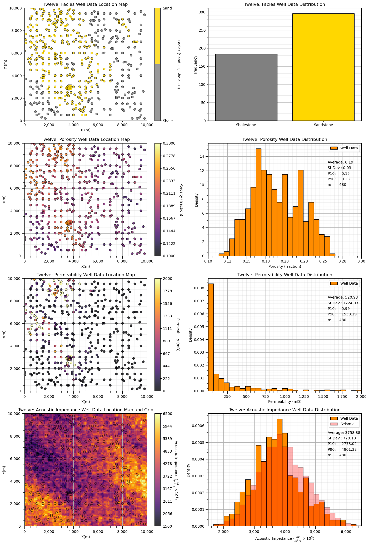
Dataset: Twelve / 12#
Twelve (12) is a densely sampled, multivariate, spatial conventional hydrocarbon dataset with large sandstone and shale facies and continuous porosity, permeability and acoustic impedance between facies.
Highlights - densely sampled, spatial with two facies, biased sampling and exhaustive secondary data.
‘12’ is a spatial multivariate dataset with,
multivariate sparse sample data,
Full Name |
Name |
Units |
Description |
|---|---|---|---|
X |
X |
\(m\) |
x coordinate |
Y |
Y |
\(m\) |
y coordinate |
Facies |
Facies |
indicator |
0 = shalestone, 1 = sandstone |
Porosity |
Porosity |
ratio |
effective porosity |
Permeability |
Perm |
\(mD\) |
isotropic, horizontal |
Acoustic Impedance |
AI |
\(\frac{kg}{m^2 \cdot s}\) |
interpolated from seismic |
2D regular grid map,
Full Name |
Name |
Units |
Description |
|---|---|---|---|
Acoustic Impedance |
AI |
\(\frac{kg}{m^2 \cdot s}\) |
inverted from seismic data |
Depositional Setting#
A single stratigraphic unit (average of 20 m in thickness) of weakly confined deepwater lobes, including possibly 7 lobe elements within a 2 lobe complexes. The lobe stacking includes components of retrogradation and compensation-driven avulsions, likely representing a rising sea level and associated waning sediment supply. Within the lobe elements there are petrophysical trends with decreasing porosity and permeability toward the lobe element margins, laterally and distally. The overbank, interlobe component, is low energy fine grained shalestone sourced from the mud component flow stripped from the turbidity currents and general hemipelagic deposition.

Method for Synthetic Data Generation#
Truth model / population by geostatistical simulation over a exhaustive grid of 10 m x 10 m cells with,
continuous porosity simulation with sequential Gaussian simulation with variogram range about 1/3 data extent
truncation of porosity simulation to calculate sand and shale facies for porosity continuity across facies boundaries
continuous, cosimulation with collocated cokriging Markov-Bayes simulation of permeability given the porosity realization
continuous, cosimulation with collocated cokriging Markov-Bayes simulation of acoustic impedance given the porosity realization
Sampling by,
combination of regular and random sampling with rejection sampler to promote a high sample bias (low for acoustic impedance) to calculate 2D well locations
values of collocated grid cell with error component assigned to the 2D point set
Load the Dataset#
df_12 = pd.read_csv(r"https://raw.githubusercontent.com/GeostatsGuy/GeoDataSets/master/12_sample_data.csv") # load the data from Dr. Pyrcz's GitHub repository
AI_12 = np.loadtxt(r'https://raw.githubusercontent.com/GeostatsGuy/GeoDataSets/master/12_AI.csv', delimiter=',')

xmin = 0.0; xmax = 10000.0; ymin = 0.0; ymax = 10000.0; nbin = 30         # set the data extents and number of bins for histograms
Dataset Dictionary#
Here’s a dictionary with all the information for each feature from this dataset.
twelve = {
    "Facies": {
        "min": 0,
        "max": 1,
        "colormap": "cmap_facies",
        "name": "Facies","fname": "Facies",
        "units": "Sand - 1, Shale - 0",
        "map": None,'format': 'int'
    },
    "Porosity": {
        "min": 0.1,
        "max": 0.3,
        "colormap": "inferno",
        "name": "Porosity","fname": "Porosity",
        "units": "fraction",
        "map": None,'format': 'small'
    },
    "Perm": {
        "min": 0.01,
        "max": 2000,
        "colormap": "inferno",
        "name": "Permeability","fname": "Perm",
        "units": "mD",
        "map": None,'format': 'large'
    },
    "AI": {
        "min": 1500,
        "max": 6500,
        "colormap": "inferno",
        "name": "Acoustic Impedance","fname": "AI",
        "units": r"$\frac{kg}{m^2 \cdot s} \times 10^3$",
        "map": AI_12,'format': 'large'
    },
}
Visualize the Dataset#
Now we can load and visualize the synthetic dataset.
for ifeature, feature in enumerate(twelve):                   # loop over features
    plt.subplot(len(twelve),2,(ifeature)*2+1)
    if feature == 'Facies':
        locmap_facies(df_12,'X','Y',twelve[feature]["fname"],xmin,xmax,ymin,ymax,twelve[feature]["min"],twelve[feature]["max"],
              'Twelve: ' + twelve[feature]["fname"] + ' Well Data Location Map','X (m)','Y (m)',twelve[feature]["name"] + ' (' + twelve[feature]["units"] + ')',
              cmap_facies)
    else:
        sc = GSLIB.locmap_st(df_12,'X','Y',twelve[feature]["fname"],xmin,xmax,ymin,ymax,twelve[feature]["min"],twelve[feature]["max"],
                'Twelve: ' + twelve[feature]["name"] + ' Well Data Location Map','X(m)','Y(m)',
                             twelve[feature]["name"] + ' (' + twelve[feature]["units"] + ')',twelve[feature]["colormap"]); add_grid2()
        if twelve[feature]["map"] is not None:
            im = plt.imshow(AI_12,interpolation = None,extent = [xmin,xmax,ymax,ymin],vmin=twelve[feature]["min"],vmax=twelve[feature]["max"],
                            origin='lower',aspect='auto',cmap=twelve[feature]["colormap"])
            plt.title('Twelve: ' + twelve[feature]['name'] + ' Well Data Location Map and Grid')
        fformatter = get_formatter(np.linspace(xmin,xmax,10),'large')
        plt.gca().xaxis.set_major_formatter(fformatter)
        plt.gca().yaxis.set_major_formatter(fformatter)

    plt.subplot(len(twelve),2,(ifeature)*2+2)
    if feature == 'Facies':
        hist_sand_shale(df_12,twelve[feature]["fname"],'Twelve: Facies Well Data Distribution')
    else:
        plt.hist(df_12[feature],bins=np.linspace(twelve[feature]["min"],twelve[feature]["max"],nbin),color='darkorange',edgecolor='black',
                 density=True,label='Well Data')
        plt.annotate('Average: ' + str(np.round(np.average(df_12[feature].values),2)),[0.78,0.82],xycoords='axes fraction')
        plt.annotate('St.Dev.: ' + str(np.round(np.std(df_12[feature].values),2)),[0.78,0.77],xycoords='axes fraction')
        plt.annotate('P10:     ' + str(np.round(np.percentile(df_12[feature].values,10),2)),[0.78,0.72],xycoords='axes fraction')
        plt.annotate('P90:     ' + str(np.round(np.percentile(df_12[feature].values,90),2)),[0.78,0.67],xycoords='axes fraction')
        plt.annotate('n:       ' + str(np.count_nonzero(~np.isnan(df_12[feature].values))),[0.78,0.62],xycoords='axes fraction')
        fformatter = get_formatter(df_12[feature].values,twelve[feature]["format"])
        plt.gca().xaxis.set_major_formatter(fformatter)
        plt.xlabel(twelve[feature]["name"] + ' (' + twelve[feature]["units"] + ')'); plt.xlim(twelve[feature]["min"],twelve[feature]["max"])
        plt.ylabel('Density')
        plt.title('Twelve: ' + twelve[feature]["name"] +  ' Well Data Distribution'); add_grid2()
        if twelve[feature]["map"] is not None:
            plt.hist(twelve[feature]["map"].flatten(),bins=np.linspace(twelve[feature]["min"],twelve[feature]["max"],nbin),
                     color='red',edgecolor='black',alpha=0.3,zorder=10,density=True,label='Seismic')
        plt.legend(loc='upper right')
plt.subplots_adjust(left=0.0, bottom=0.0, right=2.0, top=4.1, wspace=0.2, hspace=0.2); plt.show()
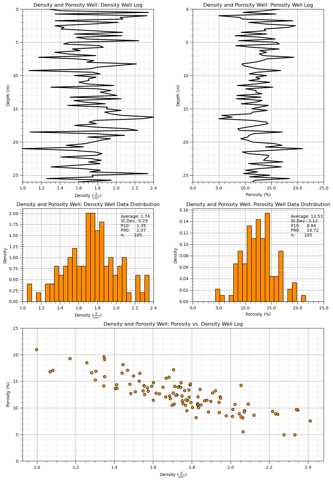
Dataset: Density and Porosity Well#
Density and Porosity Well is a single vertical well section with exhaustively sampled density from RHOB well log and porosity from a continuous well core sampled at 0.25 \(m\) intervals along the well. All of the samples are within a single reservoir formation and a single facies.
Highlights - simple 1D, 2 feature dataset with a generally linear relationship
Density and Porosity Well includes these features,
Full Name |
Name |
Units |
Description |
|---|---|---|---|
Density |
Density |
\(\frac{g}{cm^3}\) |
RHOB |
Porosity |
Porosity |
\(\%\) |
from core analysis |
Depositional Setting#
A single stratigraphic unit interpreted as stacked fluvial channel complex with channel elements from 1 to 9. The channel elements incise into each other greatly reducing the apparent element thickness and removing the low porosity top of channel element fills and overbank due to channel avulsion. The channels may be confined because of the lack of margin and overbank depofacies, the well log seems to only include the channel axis component of the stacked channel elements.

Method for Synthetic Data Generation#
Density log by,
convolution applied to a vector of random Gaussian values to impose spatial continuity
Porosity log by,
truncation of porosity simulation to calculate sand and shale facies for porosity continuity across facies boundaries
continuous, cosimulation with collocated cokriging Markov-Bayes simulation of permeability given the porosity realization
continuous, cosimulation with collocated cokriging Markov-Bayes simulation of acoustic impedance given the porosity realization
Sampling by,
combination of regular and random sampling with rejection sampler to promote a high sample bias (low for acoustic impedance) to calculate 2D well locations
values of collocated grid cell with error component assigned to the 2D point set
Load the Dataset#
df_denpor = pd.read_csv(r"https://raw.githubusercontent.com/GeostatsGuy/GeoDataSets/master/Density_Por_data.csv") # load the data from Dr. Pyrcz's GitHub repository
xmin = 0.0; xmax = 10000.0; ymin = 0.0; ymax = 10000.0; nbin = 30         # set the data extents and number of bins for histograms
Dataset Dictionary#
Here’s a dictionary with all the information for each feature from this dataset.
denpor = {
    "Depth": {
        "min": 0.0,
        "max": 26.0,
        "colormap": "inferno",
        "name": "Depth","fname": "Depth",
        "units": r"$m$",
        "map": None,'format': 'small'
    },
    "Density": {
        "min": 1.0,
        "max": 2.4,
        "colormap": "inferno",
        "name": "Density","fname": "Density",
        "units": r"$\frac{g}{cm^3}$",
        "map": None,'format': 'one'
    },
    "Porosity": {
        "min": 0.0,
        "max": 25.0,
        "colormap": "viridis",
        "name": "Porosity","fname": "Porosity",
        "units": r"$\%$",
        "map": None,'format': 'one'
    },
}
Visualize the Dataset#
Now we can load and visualize the synthetic dataset.
import matplotlib.pyplot as plt
from matplotlib.gridspec import GridSpec

feature_list = ['Density','Porosity']   # early Python does not preserve dictionary list, this is safer than looping over dictionary

fig = plt.figure(figsize=(5, 6))  # Adjust for comfortable aspect
gs = GridSpec(3, 2, height_ratios=[1.3, 0.7, 1.0], figure=fig)
ax1 = fig.add_subplot(gs[0, 0])
ax2 = fig.add_subplot(gs[0, 1])
ax3 = fig.add_subplot(gs[1, 0])
ax4 = fig.add_subplot(gs[1, 1])
ax5 = fig.add_subplot(gs[2, :])  # Spans both columns

mid_axes = [ax3,ax4]; top_axes = [ax1,ax2]

for iax, ax in enumerate(top_axes):
    feature = feature_list[iax]
    ax.plot(df_denpor[feature],df_denpor['Depth'],color='black',lw=2)
    ax.set_ylabel(denpor['Depth']["name"] + ' (' + denpor['Depth']["units"] + ')')
    ax.set_ylim(denpor['Depth']["max"],denpor['Depth']["min"]); add_grid(ax)
    ax.set_xlim(denpor[feature]["min"],denpor[feature]["max"])
    ax.set_xlabel(denpor[feature]["name"] + ' (' + denpor[feature]["units"] + ')')
    ax.set_title('Density and Porosity Well: ' + denpor[feature]["name"] + ' Well Log')
    fformatter = get_formatter(df_denpor[feature].values,denpor[feature]["format"])
    ax.xaxis.set_major_formatter(fformatter)

for iax, ax in enumerate(mid_axes):
    feature = feature_list[iax]
    ax.hist(df_denpor[feature],bins=np.linspace(denpor[feature]["min"],denpor[feature]["max"],nbin),color='darkorange',edgecolor='black',
          density=True,label='Well Data')
    ax.annotate('Average: ' + str(np.round(np.average(df_denpor[feature].values),2)),[0.75,0.90],xycoords='axes fraction')
    ax.annotate('St.Dev.: ' + str(np.round(np.std(df_denpor[feature].values),2)),[0.75,0.85],xycoords='axes fraction')
    ax.annotate('P10:     ' + str(np.round(np.percentile(df_denpor[feature].values,10),2)),[0.75,0.80],xycoords='axes fraction')
    ax.annotate('P90:     ' + str(np.round(np.percentile(df_denpor[feature].values,90),2)),[0.75,0.75],xycoords='axes fraction')
    ax.annotate('n:       ' + str(np.count_nonzero(~np.isnan(df_denpor[feature].values))),[0.75,0.70],xycoords='axes fraction')
    fformatter = get_formatter(df_denpor[feature].values,denpor[feature]["format"])
    ax.xaxis.set_major_formatter(fformatter)
    ax.set_xlabel(denpor[feature]["name"] + ' (' + denpor[feature]["units"] + ')'); ax.set_xlim(denpor[feature]["min"],denpor[feature]["max"])
    ax.set_ylabel('Density')
    ax.set_title('Density and Porosity Well: ' + denpor[feature]["name"] +  ' Well Data Distribution'); add_grid(ax)

ax5.scatter(df_denpor['Density'],df_denpor['Porosity'],color='darkorange',edgecolor='black',s=40,marker='o')
ax5.set_ylabel(denpor['Porosity']["name"] + ' (' + denpor['Porosity']["units"] + ')')
ax5.set_ylim(denpor['Porosity']["min"],denpor['Porosity']["max"]); add_grid(ax5)
ax5.set_xlabel(denpor['Density']["name"] + ' (' + denpor['Density']["units"] + ')')
ax5.set_title('Density and Porosity Well: ' + denpor['Porosity']["name"] + ' vs. ' + denpor['Density']["name"] + ' Well Log')

plt.subplots_adjust(left=0.0, bottom=0.0, right=2.0, top=2.5, wspace=0.3, hspace=0.2); plt.show()
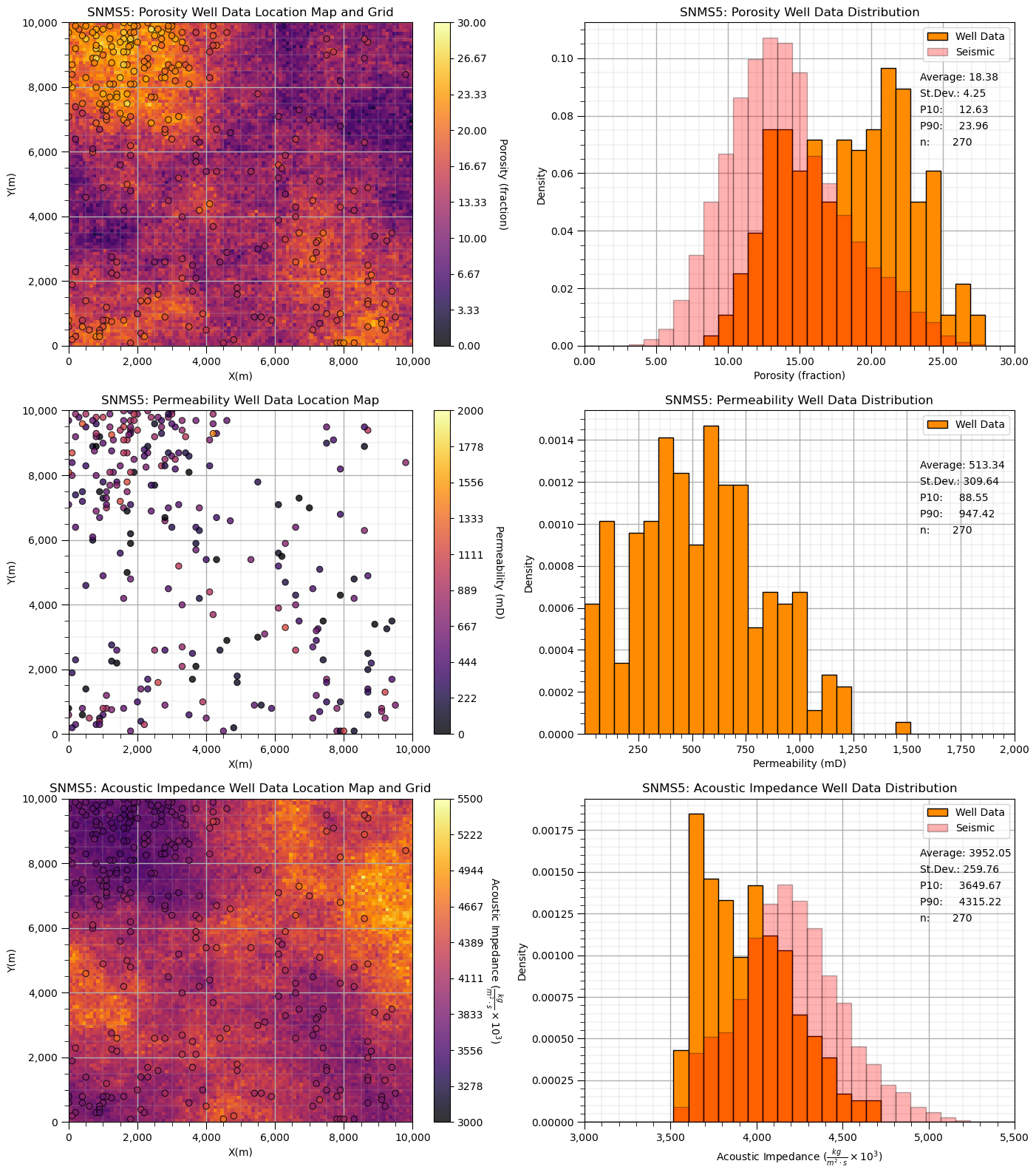
Dataset: Spatial Nonlinear Multivariate Sandstone Only Facies v5#
Spatial Nonlinear Multivariate Sandstone Only Facies v5 (SNMSv5) is a densely sampled, multivariate, spatial conventional hydrocarbon dataset with a single sandstone facies.
Link - the dataset is available here and the acoustic impedance map is here and the porosity truth model is here.
Highlights- porosity truth model for testing, missing component of the distribution suitable for soft data debiasing methods
multivariate sparse sample data,
Full Name |
Name |
Units |
Description |
|---|---|---|---|
X |
X |
\(m\) |
x coordinate |
Y |
Y |
\(m\) |
y coordinate |
Facies |
Facies |
indicator |
0 = shalestone, 1 = sandstone |
Porosity |
Porosity |
ratio |
effective porosity |
Permeability |
Perm |
\(mD\) |
isotropic, horizontal |
Acoustic Impedance |
AI |
\(\frac{kg}{m^2 \cdot s}\) |
interpolated from seismic |
2D regular grid truth model and map,
Full Name |
Name |
Units |
Description |
|---|---|---|---|
Porosity |
Porosity |
ratio |
truth model for testing |
Acoustic Impedance |
AI |
\(\frac{kg}{m^2 \cdot s}\) |
inverted from seismic data |
Depositional Setting#
A single stratigraphic unit interpreted as fluvial dominated mixed sediment delta with 2 protruding subdeltas. Within each delta and subdelta there is distributary paleoflow resulting in multiple paleoflow directions and a general reduction in porosity and permeability from inner to outer delta.

Method for Synthetic Data Generation#
Truth model / population by geostatistical simulation over a exhaustive grid of 10 m x 10 m cells with,
continuous porosity simulation with sequential Gaussian simulation with variogram range about 1/3 data extent
truncation of porosity simulation to calculate sand and shale facies for porosity continuity across facies boundaries
continuous, cosimulation with collocated cokriging Markov-Bayes simulation of permeability given the porosity realization
continuous, cosimulation with collocated cokriging Markov-Bayes simulation of acoustic impedance given the porosity realization
Sampling by,
combination of regular and random sampling with rejection sampler to promote a high sample bias (low for acoustic impedance) to calculate 2D well locations
values of collocated grid cell with error component assigned to the 2D point set
Load the Dataset and Truth Model#
df_snms5 = pd.read_csv(r"https://raw.githubusercontent.com/GeostatsGuy/GeoDataSets/master/spatial_nonlinear_MV_facies_v5_sand_only.csv") # load the data from Dr. Pyrcz's GitHub repository
AI_snms5 = np.loadtxt(r'https://raw.githubusercontent.com/GeostatsGuy/GeoDataSets/master/spatial_nonlinear_MV_facies_v5_sand_only_truth_AI.csv', delimiter=',')
Por_snms5 = np.loadtxt(r'https://raw.githubusercontent.com/GeostatsGuy/GeoDataSets/master/spatial_nonlinear_MV_facies_v5_sand_only_truth_por.csv', delimiter=',')

xmin = 0.0; xmax = 10000.0; ymin = 0.0; ymax = 10000.0; nbin = 30         # set the data extents and number of bins for histograms
Dataset Dictionary#
Here’s a dictionary with all the information for each feature from this dataset.
snms5 = {
    "Porosity": {
        "min": 0.0,
        "max": 30.0,
        "colormap": "inferno",
        "name": "Porosity","fname": "Por",
        "units": "fraction",
        "map": Por_snms5,'format': 'small'
    },
    "Perm": {
        "min": 0.01,
        "max": 2000,
        "colormap": "inferno",
        "name": "Permeability","fname": "Perm",
        "units": "mD",
        "map": None,'format': 'large'
    },
    "AI": {
        "min": 3000,
        "max": 5500,
        "colormap": "inferno",
        "name": "Acoustic Impedance","fname": "AI",
        "units": r"$\frac{kg}{m^2 \cdot s} \times 10^3$",
        "map": AI_snms5,'format': 'large'
    },
}
Visualize the Dataset#
Now we can load and visualize the synthetic dataset.
for ifeature, feature in enumerate(snms5):
    plt.subplot(len(snms5),2,(ifeature)*2+1)
    if feature == 'Facies':
        locmap_facies(df_snms5,'X','Y',snms5[feature]["fname"],xmin,xmax,ymin,ymax,twelve[feature]["min"],snms5[feature]["max"],
              'SNMS5: ' + snms5[feature]["fname"] + ' Well Data Location Map','X (m)','Y (m)',snms5[feature]["name"] + ' (' + snms5[feature]["units"] + ')',
              cmap_facies)
    else:
        sc = GSLIB.locmap_st(df_snms5,'X','Y',snms5[feature]["fname"],xmin,xmax,ymin,ymax,snms5[feature]["min"],snms5[feature]["max"],
                'SNMS5: ' + snms5[feature]["name"] + ' Well Data Location Map','X(m)','Y(m)',
                             snms5[feature]["name"] + ' (' + snms5[feature]["units"] + ')',snms5[feature]["colormap"]); add_grid2()
        if snms5[feature]["map"] is not None:
            im = plt.imshow(snms5[feature]["map"],interpolation = None,extent = [xmin,xmax,ymax,ymin],vmin=snms5[feature]["min"],vmax=snms5[feature]["max"],
                            origin='lower',aspect='auto',cmap=snms5[feature]["colormap"])
            plt.title('SNMS5: ' + snms5[feature]['name'] + ' Well Data Location Map and Grid')
        fformatter = get_formatter(np.linspace(xmin,xmax,10),'large')
        plt.gca().xaxis.set_major_formatter(fformatter)
        plt.gca().yaxis.set_major_formatter(fformatter)

    plt.subplot(len(snms5),2,(ifeature)*2+2)
    if feature == 'Facies':
        hist_sand_shale(df_snms5[feature]["map"],snms5[feature]["fname"],'Twelve: Facies Well Data Distribution')
    else:
        plt.hist(df_snms5[snms5[feature]["fname"]],bins=np.linspace(snms5[feature]["min"],snms5[feature]["max"],nbin),color='darkorange',edgecolor='black',
                 density=True,label='Well Data')
        plt.annotate('Average: ' + str(np.round(np.average(df_snms5[snms5[feature]["fname"]].values),2)),[0.78,0.82],xycoords='axes fraction')
        plt.annotate('St.Dev.: ' + str(np.round(np.std(df_snms5[snms5[feature]["fname"]].values),2)),[0.78,0.77],xycoords='axes fraction')
        plt.annotate('P10:     ' + str(np.round(np.percentile(df_snms5[snms5[feature]["fname"]].values,10),2)),[0.78,0.72],xycoords='axes fraction')
        plt.annotate('P90:     ' + str(np.round(np.percentile(df_snms5[snms5[feature]["fname"]].values,90),2)),[0.78,0.67],xycoords='axes fraction')
        plt.annotate('n:       ' + str(np.count_nonzero(~np.isnan(df_snms5[snms5[feature]["fname"]].values))),[0.78,0.62],xycoords='axes fraction')
        fformatter = get_formatter(df_snms5[snms5[feature]["fname"]].values,snms5[feature]["format"])
        plt.gca().xaxis.set_major_formatter(fformatter)
        plt.xlabel(snms5[feature]["name"] + ' (' + snms5[feature]["units"] + ')'); plt.xlim(snms5[feature]["min"],snms5[feature]["max"])
        plt.ylabel('Density')
        plt.title('SNMS5: ' + snms5[feature]["name"] +  ' Well Data Distribution'); add_grid2()
        if snms5[feature]["map"] is not None:
            plt.hist(snms5[feature]["map"].flatten(),bins=np.linspace(snms5[feature]["min"],snms5[feature]["max"],nbin),
                     color='red',edgecolor='black',alpha=0.3,zorder=10,density=True,label='Seismic')
        plt.legend(loc='upper right')
plt.subplots_adjust(left=0.0, bottom=0.0, right=2.0, top=3.1, wspace=0.2, hspace=0.2); plt.show()
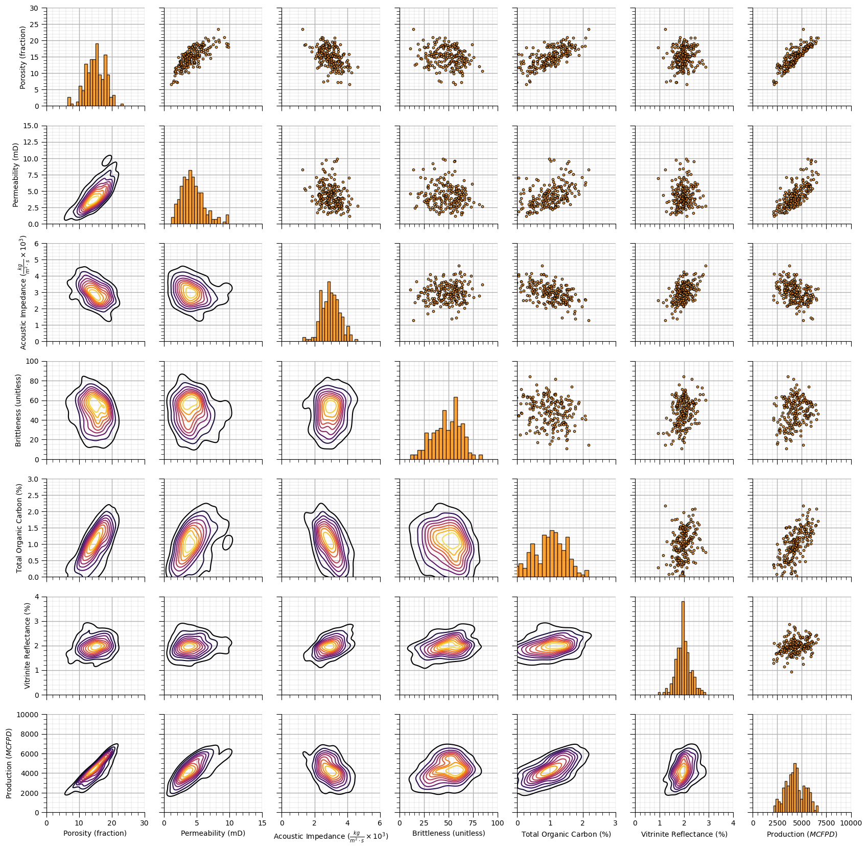
Dataset: Unconventional Multivariate v5#
Unconventional Mutlivariate v5 (UNMV5) is a densely sampled, multivariate, unconventional hydrocarbon dataset with a single sandstone facies.
Link - the dataset is available here.
Highlights - large number of potential features for feature selection, feature engineering and predictive machine learning model construction
multivariate sparse sample data,
Full Name |
Name |
Units |
Description |
|---|---|---|---|
Porosity |
Porosity |
ratio |
effective porosity |
Permeability |
Perm |
\(mD\) |
isotropic, horizontal |
Acoustic Impedance |
AI |
\(\frac{kg}{m^2 \cdot s}\) |
interpolated from seismic inversion |
Brittleness Index |
Brittle |
ratio |
elastic moduli-based method |
Total Organic Carbon |
TOC |
\(\%\) |
LECO analyzer |
Vitrinite Reflectance |
VR |
\(\%\) |
mean random reflectance |
Depositional Setting#
Mixed carbonate and siliciclastic unconventional gas reservoir with good porosity, but poor permeability. In an effort to improve production potential prediction, various features have been collected including total organic carbon, brittleness and vitrinite reflectance. Due to the complicated recovery mechanisms, and the superposition of factors such as natural fracture systems interacting with artificial fractures, and often limited matrix flow rates, unconventional reservoir forecasting can be quite challenging.
Method for Synthetic Data Generation#
Samples drawn from multivariate distributions,
sample from a large \(M\) multivariate Gaussian distribution with correlation defined by a covariance matrix with strong and weak, positive and negative correlations
calculate the features as combinations of the \(M\) features with a variety of transformations to impose nonlinear relationships
transform the marginal distributions to impose nonGaussian univariate distributions
Load the Dataset and Truth Model#
df_unmv5 = pd.read_csv(r"https://raw.githubusercontent.com/GeostatsGuy/GeoDataSets/master/unconv_MV_v5.csv") # load the data from Dr. Pyrcz's GitHub repository

nbin = 30                                # set the data extents and number of bins for histograms
Dataset Dictionary#
Here’s a dictionary with all the information for each feature from this dataset.
unmv5 = {
    "Porosity": {
        "min": 0.0,
        "max": 30.0,
        "colormap": "inferno",
        "name": "Porosity","fname": "Por",
        "units": "fraction",
        "map": None,'format': 'small'
    },
    "Perm": {
        "min": 0.0,
        "max": 15.0,
        "colormap": "inferno",
        "name": "Permeability","fname": "Perm",
        "units": "mD",
        "map": None,'format': 'large'
    },
    "AI": {
        "min": 0.0,
        "max": 6.0,
        "colormap": "inferno",
        "name": "Acoustic Impedance","fname": "AI",
        "units": r"$\frac{kg}{m^2 \cdot s} \times 10^3$",
        "map": None,'format': 'small'
    },
    "Brittle": {
        "min": 0.0,
        "max": 100,
        "colormap": "inferno",
        "name": "Brittleness","fname": "Brittle",
        "units": r"unitless",
        "map": None,'format': 'small'
    },
    "TOC": {
        "min": 0.0,
        "max": 3.0,
        "colormap": "inferno",
        "name": "Total Organic Carbon","fname": "TOC",
        "units": r"$\%$",
        "map": None,'format': 'small'
    },
    "VR": {
        "min": 0.0,
        "max": 4.0,
        "colormap": "inferno",
        "name": "Vitrinite Reflectance","fname": "VR",
        "units": r"$\%$",
        "map": None,'format': 'small'
    },
    "Prod": {
        "min": 0.0,
        "max": 10000.0,
        "colormap": "inferno",
        "name": "Production","fname": "Prod",
        "units": r"$MCFPD$",
        "map": None,'format': 'large'
    }
}
Visualize the Dataset#
Now we can load and visualize the synthetic dataset.
features = [item['fname'] for item in unmv5.values()]
keys = list(unmv5.keys())
labels = [item['name'] + ' (' + item['units'] + ')' for item in unmv5.values()]
pp_unmv5 = sns.PairGrid(df_unmv5,vars=features)
pp_unmv5 = pp_unmv5.map_upper(plt.scatter, color = 'darkorange', edgecolor = 'black', alpha = 0.8, s = 10)
pp_unmv5 = pp_unmv5.map_diag(plt.hist, bins = 20, color = 'darkorange',alpha = 0.8, edgecolor = 'k')# Map a density plot to the lower triangle
pp_unmv5 = pp_unmv5.map_lower(sns.kdeplot, cmap = plt.cm.inferno,
                              shade = False, shade_lowest = False, alpha = 1.0, n_levels = 10)

# pp_unmv5.map(sns.scatterplot)

# Draw everything first so axes exist and are not overridden
plt.draw()

for i, ax in enumerate(pp_unmv5.axes[:, 0]):  # First column => leftmost Y axes
    ax.set_ylabel(labels[i])
for i, ax in enumerate(pp_unmv5.axes[-1, :]):  # First column => leftmost Y axes
    ax.set_xlabel(labels[i])
for i in range(len(pp_unmv5.axes)):
    for j in range(len(pp_unmv5.axes)):
        # print(i,j)
        ax = pp_unmv5.axes[i, j]
        ax.set_xlim(unmv5[keys[j]]["min"],unmv5[keys[j]]["max"])
        ax.set_ylim(unmv5[keys[i]]["min"],unmv5[keys[i]]["max"])
        add_grid(ax)

plt.subplots_adjust(left=0.0, bottom=0.0, right=0.9, top=0.9, wspace=0.2, hspace=0.2); plt.show()
Dataset: Reservoir 21#
Reservoir 21 is a large, isolated reservoir unit with good porosity and permeability.
Depositional Setting#
The reservoir sediments was transported by submarine turbidity currents and deposited lithified to become turbidites. The turbidites are separated into 4 ordinal facies,
shalestone
sandy-shalestone
shaly-sandstone
sandstone
with increase rock quality, porosity and permeability over the above indicated categories from worst = 1 (shalestone) to best = 4 (sandstone). Postdepositional the turbidite formation’s pore space was filled by migrating hydrocarbons that were trapped by a thick shale above the unit.
The transport and depositional mechanisms of turbidites are explained in Wikipedia’s Turbidtes Article and a good overview of modeling turbidite reservoirs is available in McHarge et al., 2011.
A schematic of turbidite transport and demposition is available in Wikipedia Turbidite article (Figure 1).
A good model for is a submarine avalanche, known as a turbidity current, traveling from the shelf break down the slope to the deep ocean basins
the driving force is a apparent increase in density due to the mixing of water and grains
the gradient of the slope is typically between 1 and 2 degrees (1% - 4% gradient)
these turbidity current can travel 100s to 1,500 km (Bay of Biscay to the Atlantic abyssal plain)
common speeds are 5 - 20 m/s (20 - 70 km/h)
to visualize this in the laboratory, see this short Turbidity Current YouTube Video.
Turbidity currents result in formation of extensive high porosity and moderate permeability reservoirs in deep water settings.
Here’s some more important details about this dataset,
Volume of Interest: clastic deepwater turbidite reservoir unit with extents 10 km by 10 km by 50 m (thickness)
Fluids: initial oil water contact is at the depth of 3067.4m and the average connate water saturation is about 20.3%
Structure: Anticline structure with a major vertical fault that crosses the reservoir (see location and equation on the image below). It is unknown if there is translation (discontinuity) across the fault.
Grids: the 2D maps conform to the standard Python convention, origin on Top Left (see the image below).
Figure 2: Plan view of Reservoir 21.
Wells: 83 vertical wells were drilled across the reservoir and completed throughout the reservoir unit. Due to the field management constraints, only 73 wells were open to produce oil for the first three years, while the remaining 10 wells were kept shut-in. At the end of the third year, the remaining 10 unproduced wells are planned to be opened.
Well Logs#
The well logs for the 73 wells are available at,
and the associated 1, 2 and 3 year cumulative oil and water production are available at,
while the new 10 wells (prior to production) well logs are available at,
Comments:
all the well names are masked (replaced with simple indices from 1 to 83) and coordinates transformed to the area of interest to conceal the actual reservoir.
available petrophysical and geomechanical properties are listed.
blank entries in the file indicate missing data at those locations.
Predictor features:
Feature |
Units |
Description |
|---|---|---|
Well ID |
Integer |
Unique well identifier, anonymized, random integer |
X, Y |
\(m\) |
Well location in area of interest (0 - 10,000 in X and Y) |
Facies |
ordinal category |
1 = shalestone, 2 = sandy-shalestone, 3 shaly-sandstone, 4 sandstone. |
Porosity |
% |
Measure of the void spaces in a material, expressed as a percentage. |
Permeability |
\(mD\) |
Ability of a material to allow fluids to pass through its pore spaces im milliDarcies. |
Acoustic Impedance |
\(kg/m^2 \cdot s x 10^6\) |
Product of a material’s density and sound velocity, affecting wave behavior. |
Rock Density |
\(g/cm^3\) |
Mass of a rock per unit volume. |
P-wave Velocity |
\(\frac{m}{s}\) |
Speed of compressional seismic waves through a material. |
S-wave Velocity |
\(\frac{m}{s}\) |
Speed of shear seismic waves through a material. |
Young’s Modulus |
\(GPa\) |
Ratio of stress to strain in the elastic region; measures stiffness in gigapascals. |
Shear Modulus |
\(GPa\) |
Ratio of shear stress to shear strain; measures resistance to shear in gigapascals. |
Response Feature:
Feature |
Units |
Description |
|---|---|---|
Cumul. Oil 1 year |
Mbbls |
Total oil produced by the well over one year in 1000s of barrels |
Cumul. Oil 2 year |
Mbbls |
Total oil produced by the well over two years in 1000s of barrels |
Cumul. Oil 3 year |
Mbbls |
Total oil produced by the well over three years in 1000s of barrels |
Cumul. Water 1 year |
Mbbls |
Total water produced by the well over one year in 1000s of barrels |
Cumul. Water 2 year |
Mbbls |
Total water produced by the well over two years in 1000s of barrels |
Cumul. Water 3 year |
Mbbls |
Total water produced by the well over three year in 1000s of barrels |
Map Data#
The following map data are available,
Acoustic impedance (AI) inverted from geophysical amplitudes and interpretations,
Proportion of facies, sandstone, shaly-sandstone, sandy-shalestone and shalestone are available at,
Note, the facies proportions are calculated by a well calibrated model with well data and acoustic impedance and the 4 proportions sum to 1.0 (honor probability closure). The top of the formation map is available at,
Comments on the 2D map, gridded data format,
2D maps are regular grids 200 by 200 cells, cell extents are 50m by 50m, extending over the reservoir
values indicate the vertically averaged property, vertical resolution is the entire reservoir unit
the indices follow standard Python convention, original is top left corner, indices are from 0, 1, …, n-1 and the first index is the row (from the top) and the second index is the column from the left
e.g. to select the 5th grid cell in x (column) and the 10th grid cell in y (rows), use ndarray[9,4] in Python (aside, array[10,5] in Matlab)
the origin of the 2D data (e.g., array[0,0]) is the center of the top left cell, 25m and 25m along y and x direction (refer to the image above)
2D Vertically Averaged Data#
For simplified workflow testing, a vertically averaged 2D variant of the dataset was made by,
averaging all the continuous well log features over the entire reservoir unit
combining a single response feature (3 year cumulative oil production) with the predictor features
removing facies to avoid the issue of upscaling the categorical ordinal feature
These two files contain the predictor features, well log data, averaged over the entire well bore for all 73 wells, i.e., one value per well for each feature, and the one response feature, 3 year cumulative oil production,
res21_2D_wells.csv - 2D averaged well data and 3 year cumulative oil production for the previous production wells, well indices from 1 to 73
and well log data averaged over the entire well bore for all 10 test wells,
res21_2D_wells_test.csv - 2D averaged well data for the remaining, preproduction wells, well indices from 74 to 83
res21 = {
    "X": {
        "min": 0.0,
        "max": 10000.0,
        "colormap": "inferno",
        "name": "X","fname": "X",
        "units": "m",
        "map": None,'format': 'small'
    },
    "Y": {
        "min": 0.0,
        "max": 10000.0,
        "colormap": "inferno",
        "name": "Y","fname": "Y",
        "units": "m",
        "map": None,'format': 'small'
    },
    "Por": {
        "min": 10.0,
        "max": 17.0,
        "colormap": "inferno",
        "name": "Porosity","fname": "Por",
        "units": "%",
        "map": None,'format': 'small'
    },
    "Perm": {
        "min": 70.0,
        "max": 200.0,
        "colormap": "inferno",
        "name": "Permeability","fname": "Perm",
        "units": "mD",
        "map": None,'format': 'large'
    },
    "AI": {
        "min": 6.9,
        "max": 7.6,
        "colormap": "inferno",
        "name": "Acoustic Impedance","fname": "AI",
        "units": r"$\frac{kg}{m^2 \cdot s} \times 10^3$",
        "map": None,'format': 'small'
    },
    "Density": {
        "min": 1.6,
        "max": 2.6,
        "colormap": "inferno",
        "name": "Density","fname": "Density",
        "units": r"\frac{g}{cm^2}",
        "map": None,'format': 'small'
    },
    "PVel": {
        "min": 3200.0,
        "max": 4500.0,
        "colormap": "inferno",
        "name": "P-wave Velocity","fname": "PVel",
        "units": r"$\frac{m}{s}$",
        "map": None,'format': 'small'
    },
    "Youngs": {
        "min": 22.0,
        "max": 32.0,
        "colormap": "inferno",
        "name": "Youngs Modulas","fname": "Youngs",
        "units": r"$GPA$",
        "map": None,'format': 'small'
    },
    "SVel": {
        "min": 1600.0,
        "max": 1750.0,
        "colormap": "inferno",
        "name": "S-wave Velocity","fname": "SVel",
        "units": r"$\frac{m}{s}$",
        "map": None,'format': 'small'
    },
    "Shear": {
        "min": 4.5,
        "max": 7.0,
        "colormap": "inferno",
        "name": "Shear Modulus","fname": "Shear",
        "units": r"$GPA$",
        "map": None,'format': 'small'
    },
    "CumulativeOil": {
        "min": 0.0,
        "max": 3000.0,
        "colormap": "inferno",
        "name": "Cumulative Oil Production","fname": "CumulativeOil",
        "units": r"$Mbbls$",
        "map": None,'format': 'large'
    }
}
Load the Dataset and Truth Model#
Let’s load the 2D dataset and visualize it.
df_res21_2D = pd.read_csv(r"https://raw.githubusercontent.com/GeostatsGuy/GeoDataSets/refs/heads/master/res21_2D_wells.csv", index_col='Well_ID') # load the data from Dr. Pyrcz's GitHub repository
df_res21_2D_test = pd.read_csv(r"https://raw.githubusercontent.com/GeostatsGuy/GeoDataSets/refs/heads/master/res21_2D_wells_test.csv", index_col='Well_ID') # load the data from Dr. Pyrcz's GitHub repository
#df_res21_2D.head()                                           # vizualize dataframe with 73 wells without production
#df_res21_2D_test.head()                                      # visualize dataframe with 10 wells with production
df_res21_2D.describe().transpose()                            # check summary statistics
| count | mean | std | min | 25% | 50% | 75% | max | |
|---|---|---|---|---|---|---|---|---|
| X | 73.0 | 4188.698630 | 1783.143687 | 1175.000000 | 2925.000000 | 3875.000000 | 5325.000000 | 7975.000000 |
| Y | 73.0 | 5770.890411 | 2405.487844 | 775.000000 | 3825.000000 | 6125.000000 | 7625.000000 | 9775.000000 |
| Por | 69.0 | 12.822361 | 1.069242 | 10.449132 | 12.122789 | 12.842228 | 13.532038 | 15.837603 |
| Perm | 53.0 | 119.292589 | 23.003770 | 85.457752 | 101.821216 | 116.341824 | 130.554974 | 184.753428 |
| AI | 69.0 | 7.319194 | 0.096761 | 7.062172 | 7.280405 | 7.333877 | 7.379185 | 7.499137 |
| Density | 70.0 | 2.043288 | 0.138222 | 1.793870 | 1.921390 | 2.039170 | 2.162651 | 2.301552 |
| PVel | 69.0 | 3696.762373 | 276.382117 | 3229.902892 | 3463.035301 | 3688.453880 | 3897.219799 | 4327.857887 |
| Youngs | 49.0 | 27.173417 | 2.164984 | 23.516002 | 25.378138 | 26.801655 | 28.641350 | 31.463424 |
| SVel | 65.0 | 1676.908144 | 19.277228 | 1637.806458 | 1662.280505 | 1676.458624 | 1688.682882 | 1721.987891 |
| Shear | 48.0 | 5.793693 | 0.474087 | 4.937921 | 5.397281 | 5.769809 | 6.208277 | 6.714150 |
| CumulativeOil | 73.0 | 940.976027 | 429.622150 | 307.120000 | 643.140000 | 819.490000 | 1185.400000 | 2514.500000 |
Now let’s load two of the 2D maps,
average sand proportion
acoustic impedance
sand_prop_map_url = requests.get('https://raw.githubusercontent.com/GeostatsGuy/GeoDataSets/refs/heads/master/res21_2d_sand_prop_map.npy')
sand_prop_map_url.raise_for_status()                          # Raise an error if the download fails
sand_prop_map = np.load(BytesIO(sand_prop_map_url.content))   # load the .npy file from the downloaded bytes

AI_map_url = requests.get('https://raw.githubusercontent.com/GeostatsGuy/GeoDataSets/refs/heads/master/res21_ai_map.npy')
AI_map_url.raise_for_status()                                 # Raise an error if the download fails
AI_map = np.load(BytesIO(AI_map_url.content))                 # load the .npy file from the downloaded bytes
AI_map = AI_map/1000000.0
Calculate Histograms for Each Feature#
Let’s use the dictionary above to make histograms for each feature.
for ifeat,feature in enumerate(df_res21_2D.columns):          # loop over all features in the dataframe with 73 wells with production
    plt.subplot(4,3,ifeat+1)                                  # subplot
    plt.hist(df_res21_2D[res21[feature]['fname']],bins=np.linspace(res21[feature]['min'],res21[feature]['max'],nbin), # histogram
             color='darkorange',edgecolor='black')
    plt.xlabel(res21[feature]['name'] + ' (' + res21[feature]['units'] +')'); plt.ylabel('Frequency'); plt.title(feature + ' Histogram') # labels
    add_grid2()                                               # major and minor gridlines function

plt.subplots_adjust(left=0.0, bottom=0.0, right=3.0, top=3.1, wspace=0.2, hspace=0.25); plt.show()
Visualize the Dataset#
Now we can visualize the synthetic dataset.
ifeat = 4                                                    # select feature for scatter plot, 0 - 10
feature =  list(res21)[ifeat]

plt.subplot(121)
im = plt.imshow(sand_prop_map,extent=[0,10000,10000,0],vmin=0,vmax=0.50,cmap=cmap) # 2D map
cb1 = plt.colorbar(im, fraction=0.036, pad=0.18)                         # colorbar for 2D map
cb1.set_label("Proportion of Sand (fraction)")                           # colorbar label for 2D map

sc = plt.scatter(df_res21_2D['X'],df_res21_2D['Y'],c=df_res21_2D[res21[feature]['fname']],s=30,edgecolor='black',
            vmin=res21[feature]['min'],vmax=res21[feature]['max'],cmap=cmap,label='current wells')       # wells with production scatter plot
cb2 = plt.colorbar(sc, fraction=0.046, pad=0.02)                         # colorbar for scatter plot
cb2.set_label(res21[feature]['name'] + ' (' + res21[feature]['units'] +')') # colorbar label for scatter plot

plt.scatter(df_res21_2D_test['X'],df_res21_2D_test['Y'],color='white',s=30,edgecolor='black',label='new wells') # wells without production
plt.xlabel('X (m)'); plt.ylabel('Y (m)'); plt.title(res21[feature]['name'] + ' and Sand Proportion Map') # labels for axes and title
plt.tight_layout(); plt.legend(loc='upper right')

plt.subplot(122)
im = plt.imshow(AI_map,extent=[0,10000,10000,0],vmin=res21['AI']['min'],vmax=res21['AI']['max'],cmap=cmap) # 2D map
cb1 = plt.colorbar(im, fraction=0.036, pad=0.18)                         # colorbar for 2D map
cb1.set_label(res21['AI']['name'] + ' (' + res21['AI']['units'] +')')                           # colorbar label for 2D map

sc = plt.scatter(df_res21_2D['X'],df_res21_2D['Y'],c=df_res21_2D[res21[feature]['fname']],s=30,edgecolor='black',
            vmin=res21[feature]['min'],vmax=res21[feature]['max'],cmap=cmap,label='current wells') # wells with production scatter plot
cb2 = plt.colorbar(sc, fraction=0.046, pad=0.02)                         # colorbar for scatter plot
cb2.set_label(res21[feature]['name'] + ' (' + res21[feature]['units'] +')') # colorbar label for scatter plot

plt.scatter(df_res21_2D_test['X'],df_res21_2D_test['Y'],color='white',s=30,edgecolor='black',label='new wells') # wells without production
plt.xlabel('X (m)'); plt.ylabel('Y (m)'); plt.title(res21[feature]['name'] + ' and Acoustic Impedance Map') # labels for axes and title
plt.tight_layout(); plt.legend(loc='upper right')

plt.subplots_adjust(left=0.0, bottom=0.0, right=2.0, top=1.1, wspace=0.3, hspace=0.25); plt.show()
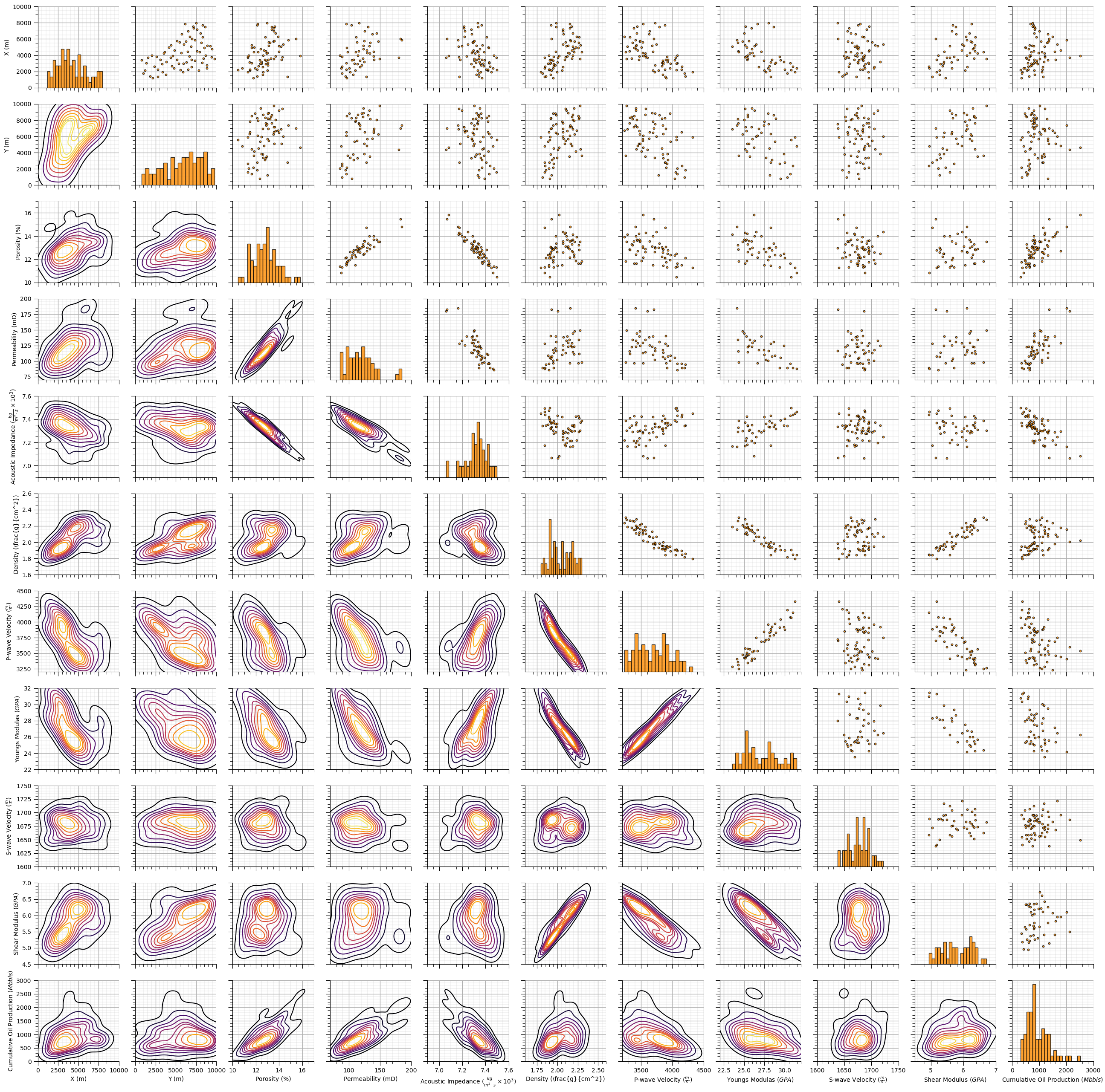
Scatter Plots#
Let’s check the relationships between the features.
features = [item['fname'] for item in res21.values()]
keys = list(res21.keys())
labels = [item['name'] + ' (' + item['units'] + ')' for item in res21.values()]
pp_res21 = sns.PairGrid(df_res21_2D,vars=features)
pp_res21 = pp_res21.map_upper(plt.scatter, color = 'darkorange', edgecolor = 'black', alpha = 0.8, s = 10)
pp_res21 = pp_res21.map_diag(plt.hist, bins = 20, color = 'darkorange',alpha = 0.8, edgecolor = 'k')# Map a density plot to the lower triangle
pp_res21 = pp_res21.map_lower(sns.kdeplot, cmap = plt.cm.inferno,
                              shade = False, shade_lowest = False, alpha = 1.0, n_levels = 10)

# Draw everything first so axes exist and are not overridden
plt.draw()

for i, ax in enumerate(pp_res21.axes[:, 0]):  # First column => leftmost Y axes
    ax.set_ylabel(labels[i])
for i, ax in enumerate(pp_res21.axes[-1, :]):  # First column => leftmost Y axes
    ax.set_xlabel(labels[i])
for i in range(len(pp_res21.axes)):
    for j in range(len(pp_res21.axes)):
        # print(i,j)
        ax = pp_res21.axes[i, j]
        ax.set_xlim(res21[keys[j]]["min"],res21[keys[j]]["max"])
        ax.set_ylim(res21[keys[i]]["min"],res21[keys[i]]["max"])
        add_grid(ax)

plt.subplots_adjust(left=0.0, bottom=0.0, right=0.9, top=0.9, wspace=0.2, hspace=0.2); plt.show()
About the Author#

Michael Pyrcz is a professor in the Cockrell School of Engineering, and the Jackson School of Geosciences, at The University of Texas at Austin, where he researches and teaches subsurface, spatial data analytics, geostatistics, and machine learning. Michael is also,
the principal investigator of the Energy Analytics freshmen research initiative and a core faculty in the Machine Learn Laboratory in the College of Natural Sciences, The University of Texas at Austin
an associate editor for Computers and Geosciences, and a board member for Mathematical Geosciences, the International Association for Mathematical Geosciences.
Michael has written over 70 peer-reviewed publications, a Python package for spatial data analytics, co-authored a textbook on spatial data analytics, Geostatistical Reservoir Modeling and author of two recently released e-books, Applied Geostatistics in Python: a Hands-on Guide with GeostatsPy and Applied Machine Learning in Python: a Hands-on Guide with Code.
All of Michael’s university lectures are available on his YouTube Channel with links to 100s of Python interactive dashboards and well-documented workflows in over 40 repositories on his GitHub account, to support any interested students and working professionals with evergreen content. To find out more about Michael’s work and shared educational resources visit his Website.
Want to Work Together?#
I hope this content is helpful to those that want to learn more about subsurface modeling, data analytics and machine learning. Students and working professionals are welcome to participate.
Want to invite me to visit your company for training, mentoring, project review, workflow design and / or consulting? I’d be happy to drop by and work with you!
Interested in partnering, supporting my graduate student research or my Subsurface Data Analytics and Machine Learning consortium (co-PI is Professor John Foster)? My research combines data analytics, stochastic modeling and machine learning theory with practice to develop novel methods and workflows to add value. We are solving challenging subsurface problems!
I can be reached at mpyrcz@austin.utexas.edu.
I’m always happy to discuss,
Michael
Michael Pyrcz, Ph.D., P.Eng. Professor, Cockrell School of Engineering and The Jackson School of Geosciences, The University of Texas at Austin
More Resources Available at: Twitter | GitHub | Website | GoogleScholar | Geostatistics Book | YouTube | Applied Geostats in Python e-book | Applied Machine Learning in Python e-book | LinkedIn
Comments#
This is a summary of some of the synthetic datasets that I have generated for the demonstrations in the e-book and my other course content. I hope this,
helps you better understand the datasets used in this book
provides some other datasets for your to test your knowledge and to benchmark your workflows
I hope this is helpful,
Michael